Beyond the Basics: Mastering the Beer-Lambert Law for Robust Quantitative Analysis in Biomedical Research

Abstract

This article provides a comprehensive resource for researchers and drug development professionals on the application of the Beer-Lambert Law in quantitative spectrophotometry. It moves from foundational principles, explaining the law's mathematical formulation and key components like absorbance and molar absorptivity, to practical methodologies for concentration determination and calibration curves. Crucially, it addresses common limitations and deviations—such as those caused by high concentrations, scattering in biological matrices, and chemical interactions—offering troubleshooting strategies and optimization techniques. Finally, the article covers validation protocols essential for regulatory compliance and explores advanced modifications and comparative data analysis methods, including machine learning, that enhance the law's utility for complex, real-world samples like blood and tissues.

The Core Principles: Deconstructing the Beer-Lambert Law for Quantitative Analysis

In the realm of quantitative analysis research, the Beer-Lambert law serves as the foundational principle enabling scientists to determine analyte concentrations through light absorption measurements. This empirical law bridges the gap between a material's molecular properties and its interaction with electromagnetic radiation, providing researchers in drug development and analytical chemistry with powerful tools for substance quantification. At the core of the Beer-Lambert law lie two fundamental optical concepts: transmittance and absorbance. These interrelated quantities describe how light propagates through matter, with their logarithmic relationship forming the mathematical basis for most modern spectroscopic techniques. The precision of concentration measurements in pharmaceutical analysis, environmental monitoring, and clinical diagnostics directly depends on accurately understanding and applying this conceptual framework.

Fundamental Definitions: Transmittance and Absorbance

Transmittance

Transmittance (T) quantifies the fraction of incident light that passes through a sample material. When monochromatic light with an initial intensity ((I_0)) enters a sample, and light with intensity ((I)) exits on the other side, transmittance is defined as the ratio of these two intensities [1] [2]:

[ T = \frac{I}{I_0} ]

Transmittance is a dimensionless quantity with values ranging from 0 to 1, though it is frequently expressed as a percentage (%T) ranging from 0% to 100% [1]. A transmittance of 1 (or 100%) indicates that all incident light passes through the sample without any absorption or scattering, while a transmittance of 0 (0%) signifies complete attenuation where no light emerges from the sample [3].

Absorbance

Absorbance (A) represents the logarithm of the reciprocal of transmittance, providing a quantitative measure of how much light a sample absorbs at a specific wavelength [2] [3]:

[ A = \log{10}\left(\frac{I0}{I}\right) = -\log{10}(T) = \log{10}\left(\frac{1}{T}\right) ]

Unlike transmittance, absorbance has no upper limit, though values between 0.1 and 1 are typically ideal for analytical measurements [2]. An absorbance of 0 corresponds to 100% transmittance (no absorption), while an absorbance of 1 indicates 10% transmittance (90% absorption) [1]. This logarithmic scale makes absorbance directly proportional to the concentration of the absorbing species, as articulated in the Beer-Lambert law.

The Logarithmic Relationship and its Mathematical Foundation

Theoretical Basis

The logarithmic relationship between transmittance and absorbance stems from the fundamental physical principle that light attenuation through a homogeneous medium occurs exponentially rather than linearly. As light traverses through infinitesimally thin layers of a sample, each layer absorbs an equal fraction of the incident radiation [4]. This multiplicative absorption process naturally leads to an exponential decay of light intensity, which linearizes through logarithmic transformation [2] [4].

The transformation from the exponential domain of transmittance to the linear domain of absorbance represents a crucial mathematical convenience for quantitative analysis. While transmittance decreases geometrically with increasing concentration or path length, absorbance increases arithmetically, establishing the direct proportional relationship essential for analytical applications [1] [2].

Quantitative Relationship Table

The table below illustrates the precise mathematical relationship between absorbance and transmittance values [1]:

Absorbance (A)	Transmittance (T)	Percent Transmittance (%T)
0	1	100%
0.1	0.79	79%
0.3	0.50	50%
0.5	0.32	32%
1.0	0.1	10%
2.0	0.01	1%
3.0	0.001	0.1%
4.0	0.0001	0.01%

Table 1: Absorbance and transmittance value relationships

This inverse logarithmic relationship demonstrates why absorbance becomes the preferred quantity in analytical applications. For instance, when 90% of light is absorbed (A=1, T=0.1), doubling the concentration of the absorbing species would result in 99% absorption (A=2, T=0.01), not 180% absorption, which would be mathematically impossible [1] [3].

Mathematical Derivation

The derivation of this relationship begins with the differential form of the attenuation law. For a thin layer of thickness (dz), the decrease in radiant flux ((d\Phi_e)) is proportional to both the incident flux and the thickness [4]:

[ \frac{d\Phie(z)}{dz} = -\mu(z)\Phie(z) ]

Solving this differential equation with the boundary condition (\Phie(0) = \Phie^i) yields [4]:

[ \Phie^t = \Phie^i \exp\left(-\int_0^\ell \mu(z)dz\right) ]

where (\Phi_e^t) represents the transmitted flux through a path length (\ell). The transmittance is therefore [4]:

[ T = \frac{\Phie^t}{\Phie^i} = \exp\left(-\int_0^\ell \mu(z)dz\right) ]

Taking the base-10 logarithm of the reciprocal establishes the connection to absorbance [2] [4]:

[ A = -\log{10}(T) = \log{10}\left(\frac{\Phie^i}{\Phie^t}\right) = \frac{1}{\ln(10)}\int0^\ell \mu(z)dz \approx 0.4343\int0^\ell \mu(z)dz ]

This derivation confirms the logarithmic relationship between transmittance and absorbance while demonstrating how absorbance linearizes the exponential attenuation process.

The Beer-Lambert Law: From Theory to Application

Fundamental Principle

The Beer-Lambert law (also known as Beer's law) establishes a direct proportional relationship between absorbance and the concentration of an absorbing species [1] [2]. For a single attenuating species in a homogeneous solution, the law is mathematically expressed as [2] [3]:

[ A = \epsilon \cdot c \cdot l ]

Where:

• (A) is the measured absorbance (dimensionless)
• (\epsilon) is the molar absorptivity or molar extinction coefficient (typically in L·mol⁻¹·cm⁻¹)
• (c) is the concentration of the absorbing species (typically in mol/L or M)
• (l) is the optical path length through the sample (typically in cm)

The molar absorptivity ((\epsilon)) is a substance-specific constant that measures how strongly a chemical species absorbs light at a particular wavelength [2] [5]. This molecular property depends on both the chemical identity of the absorber and the wavelength of incident light.

Experimental Verification Methodology

Objective: To verify the linear relationship between absorbance and concentration as predicted by the Beer-Lambert law using a series of standard solutions.

Materials and Equipment:

• Spectrophotometer with appropriate wavelength selection capability
• Matched cuvettes (typically with 1.0 cm path length)
• Analytical balance
• Volumetric flasks
• Precise pipettes
• Stock solution of analyte (e.g., Rhodamine B in water)
• Solvent for dilution (e.g., deionized water)

Procedure:

• Prepare a stock solution of known concentration (e.g., 1.0×10⁻³ M Rhodamine B)
• Create a series of standard solutions through precise serial dilution (e.g., 2.0×10⁻⁴ M, 4.0×10⁻⁴ M, 6.0×10⁻⁴ M, 8.0×10⁻⁴ M, 1.0×10⁻³ M)
• Set the spectrophotometer to the wavelength of maximum absorption ((\lambda_{max})) for the analyte (e.g., 550 nm for Rhodamine B)
• Measure the blank (pure solvent) and zero the instrument
• Measure the absorbance of each standard solution in sequence, ensuring proper cuvette orientation
• Record absorbance values for each concentration

Data Analysis:

• Plot absorbance versus concentration
• Perform linear regression analysis
• Determine the correlation coefficient (R²) to assess linearity
• Calculate the molar absorptivity ((\epsilon)) from the slope of the calibration curve

Expected Results: The experiment should yield a linear calibration curve similar to published results for Rhodamine B, where absorbance at (\lambda_{max}) shows direct proportionality to concentration [1]. The slope of this curve provides the product (\epsilon \cdot l), from which (\epsilon) can be calculated knowing the path length (l).

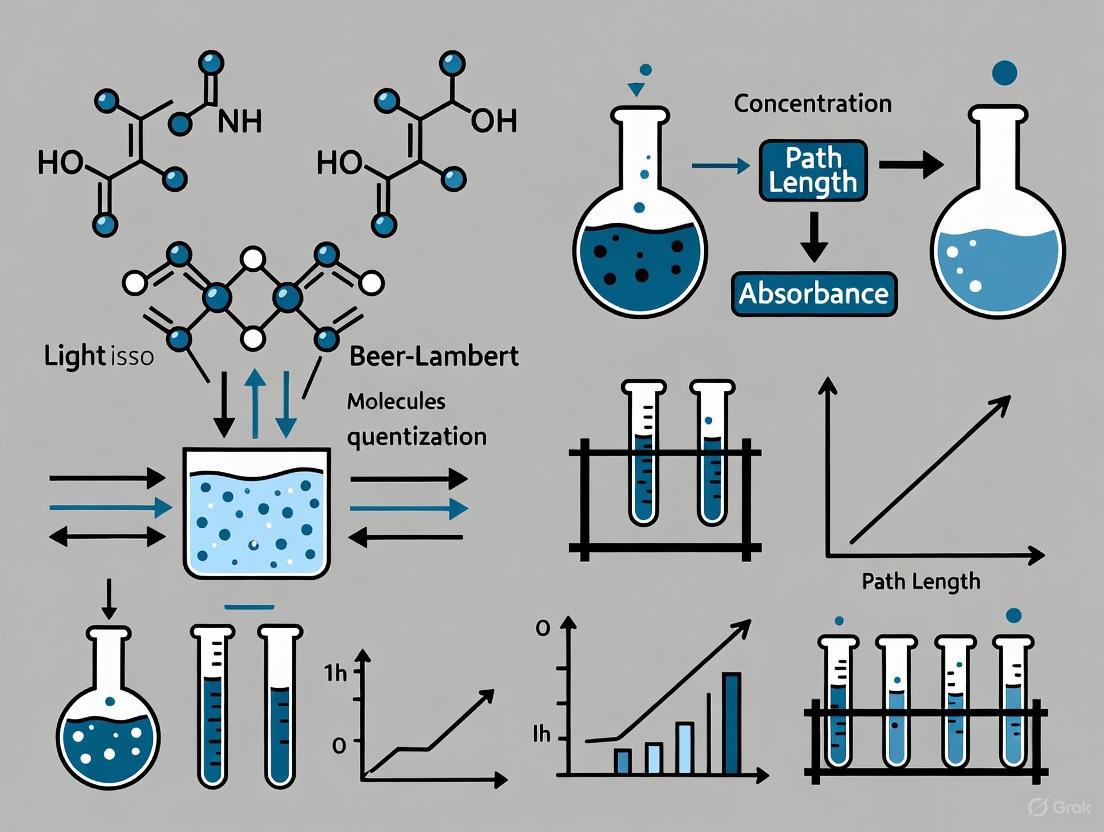
Visualizing the Beer-Lambert Law Relationship

The following diagram illustrates the core principles and experimental workflow of the Beer-Lambert law:

Diagram 1: Beer-Lambert law principles and relationships

Advanced Considerations and Practical Limitations

Deviations from Beer-Lambert Law

While the Beer-Lambert law provides an excellent foundation for quantitative analysis, several factors can cause deviations from ideal linear behavior [6] [3]:

• High Concentration Effects: At elevated concentrations (>0.01 M), intermolecular distances decrease, potentially altering absorptivity through molecular interactions or electrostatic effects [6] [3].

• Chemical Equilibria: pH-dependent equilibria (e.g., acid-base indicators) can shift species distribution, changing effective molar absorptivity [6].

• Instrumental Limitations: Stray light, polychromatic radiation, and detector non-linearity introduce measurement errors [6] [3].

• Scattering Effects: Particulate matter or turbidity causes light scattering, increasing apparent absorption [3].

• Fluorescence: Emitted light from fluorescent samples can reach the detector, reducing measured absorbance [6].

Multi-Component Analysis

For samples containing multiple absorbing species, the Beer-Lambert law becomes additive [6]:

[ A{total} = \epsilon1 \cdot c1 \cdot l + \epsilon2 \cdot c2 \cdot l + \cdots + \epsilonn \cdot c_n \cdot l ]

Quantifying individual components requires measuring absorbance at multiple wavelengths and solving simultaneous equations [6]:

[ \begin{aligned} A{\lambda1} &= \epsilon{1,\lambda1} \cdot c1 \cdot l + \epsilon{2,\lambda1} \cdot c2 \cdot l \ A{\lambda2} &= \epsilon{1,\lambda2} \cdot c1 \cdot l + \epsilon{2,\lambda2} \cdot c2 \cdot l \end{aligned} ]

Advanced mathematical approaches including derivative spectroscopy and multivariate calibration enable analysis of complex mixtures [6].

Essential Research Reagents and Materials

Successful implementation of absorption spectroscopy for quantitative analysis requires specific laboratory materials and reagents. The following table details essential components for experiments based on the Beer-Lambert law:

Category	Specific Items	Function & Importance
Instrumentation	UV-Vis Spectrophotometer	Measures intensity of light before and after sample with wavelength selection capability [3]
	Cuvettes (1 cm path length)	Contain sample solution with precise, reproducible optical path length [2]
Solvents & Buffers	High-purity solvents (H₂O, CH₃OH, CHCl₃)	Dissolve analytes without contributing significant background absorption [6]
	pH Buffer solutions	Maintain constant chemical environment to prevent shifts in absorption spectra [6]
Reference Standards	Analytical standards (e.g., Rhodamine B)	Establish calibration curves with known concentrations for quantitative analysis [1]
	Blank solutions	Contain all components except analyte to establish baseline measurements [3]
Sample Preparation	Volumetric flasks	Provide accurate volume measurements for precise concentration preparation
	Precision pipettes	Enable accurate transfer of liquid volumes for standard solution preparation
	Analytical balance	Allows precise weighing of solid standards for stock solution preparation

Table 2: Essential research reagents and materials for absorption spectroscopy

Applications in Pharmaceutical Research and Development

The logarithmic relationship between transmittance and absorbance underpins numerous critical applications in drug development:

• Concentration Determination: Quantifying API (Active Pharmaceutical Ingredient) concentration in solutions during drug formulation [5].

• Purity Assessment: Detecting impurities through characteristic absorption signatures outside expected wavelengths [5].

• Binding Studies: Monitoring ligand-receptor interactions through absorbance changes in titration experiments.

• Dissolution Testing: Tracking drug release from formulations by measuring concentration in dissolution media over time.

• Enzyme Kinetics: Following substrate depletion or product formation in enzymatic assays via absorbance changes.

The reliability of these applications fundamentally depends on properly establishing the relationship between absorbance and concentration through calibration curves, demonstrating the enduring practical significance of the transmittance-absorbance logarithmic relationship in pharmaceutical sciences.

The logarithmic relationship between transmittance and absorbance represents far more than a mathematical convenience—it forms the theoretical cornerstone for one of the most widely applied principles in analytical chemistry. By transforming the exponential nature of light attenuation into a linear relationship between absorbance and concentration, this fundamental concept enables precise quantitative analysis across diverse scientific disciplines. For drug development professionals and researchers, mastering these core principles ensures accurate implementation of spectroscopic methods, from routine quality control measurements to sophisticated research applications. As analytical technologies advance, the enduring relationship between transmittance and absorbance continues to underpin innovations in spectroscopic quantification, maintaining its central role in the scientific toolkit for quantitative analysis.

The Beer-Lambert Law (BLL), also referred to as the Beer-Lambert-Bouguer Law or simply Beer's Law, is a fundamental principle in spectroscopy that quantitatively describes the attenuation of light as it passes through a material [7]. This law establishes a linear relationship between the absorbance of light and the properties of the absorbing medium, making it indispensable for quantitative analysis across chemical, biological, and medical research [5]. The law's development spans over a century, beginning with Pierre Bouguer's 1729 work on light attenuation in the atmosphere, which established that light remaining in a collimated beam decreases exponentially with path length in a uniform medium [7]. Johann Heinrich Lambert later provided the mathematical formulation of this exponential relationship in 1760, while August Beer extended the law in 1852 to incorporate the concentration of solutions, completing the formulation we use today [7] [8].

In modern quantitative analysis research, particularly in pharmaceutical development, the Beer-Lambert Law serves as the cornerstone for determining analyte concentrations in solutions, monitoring chemical reactions, and ensuring product quality and consistency [5]. Its mathematical elegance and practical utility have ensured its enduring relevance across diverse scientific disciplines including analytical chemistry, biomedical engineering, environmental science, and materials characterization [9] [7]. The fundamental equation, A = εlc, provides researchers with a direct means to quantify concentrations of absorbing species through relatively straightforward absorbance measurements, making it one of the most widely applied relationships in spectroscopic analysis.

Fundamental Principles and Mathematical Formulation

Core Equation and Component Definitions

The Beer-Lambert Law is mathematically expressed as:

A = εlc

Where:

• A is the absorbance (also called optical density), a dimensionless quantity representing the amount of light absorbed by the sample [2] [1] [5]
• ε is the molar absorptivity or molar extinction coefficient (in L·mol⁻¹·cm⁻¹), a substance-specific constant that indicates how strongly a chemical species absorbs light at a particular wavelength [2] [5]
• l is the path length (in cm), representing the distance light travels through the solution, typically determined by the cuvette width [2] [5]
• c is the concentration of the absorbing species (in mol/L) [2] [5]

The absorbance A is defined via the incident intensity (Iâ‚€) and transmitted intensity (I) through the logarithmic relationship:

A = log₁₀(I₀/I) [2] [1]

This logarithmic relationship means that absorbance increases as transmittance decreases. The relationship between absorbance and transmittance values follows predictable patterns as shown in Table 1.

Table 1: Relationship Between Absorbance and Transmittance

Absorbance (A)	Transmittance (T)	Percent Transmittance (%T)
0	1	100%
0.3	0.5	50%
1	0.1	10%
2	0.01	1%
3	0.001	0.1%

[1]

Derivation and Theoretical Foundation

The Beer-Lambert Law can be derived by considering the differential attenuation of light passing through an infinitesimal layer of absorbing medium. The decrease in light intensity (-dI) across a thin layer of thickness dx is proportional to the incident intensity I, the concentration of absorbers c, and the thickness dx:

-dI/I = kcdx [10]

Where k is a proportionality constant. Integrating this differential equation from x = 0 to x = l (where I = Iâ‚€ at x = 0, and I = I at x = l) yields:

ln(Iâ‚€/I) = kcl [10]

Converting from natural logarithm to base-10 logarithm gives:

log₁₀(I₀/I) = εlc [2] [10]

Where ε = k/2.303 is the molar absorptivity coefficient. This derivation establishes the fundamental exponential nature of light attenuation in absorbing media and justifies the logarithmic relationship defining absorbance [10].

Figure 1: Schematic representation of light attenuation through an absorbing medium, demonstrating the fundamental relationship described by the Beer-Lambert Law

Experimental Validation and Methodologies

Standard Protocol for Quantitative Analysis

Verifying the Beer-Lambert Law and applying it for concentration determination requires meticulous experimental methodology. The following protocol outlines the essential steps for accurate spectrophotometric analysis:

Equipment and Reagents:

• High-quality spectrophotometer with wavelength selection capability [9]
• Matched quartz or optical glass cuvettes with defined path length (typically 1 cm) [5]
• Analytical balance for precise weighing [9]
• Volumetric flasks for accurate solution preparation [9]
• Pure solvent for preparing solutions [9]
• Standard reference material of known purity [9]

Procedure:

• Instrument Calibration: Perform wavelength accuracy verification using holmium oxide or didymium filters with known absorption peaks [9]. Establish baseline correction with solvent-filled cuvettes to account for background absorption and reflection losses [11].

• Standard Solution Preparation: Prepare a stock solution of the analyte at known concentration, ensuring complete dissolution. Create a series of standard solutions through serial dilution, covering the expected concentration range of samples [9]. Maintain consistent temperature and chemical environment (pH, ionic strength) across all solutions to prevent chemical deviations [11].

• Spectral Measurement: For each standard solution, measure absorbance at the wavelength of maximum absorption (λmax) determined from preliminary scans [5]. Record triplicate measurements for each concentration to assess precision. Measure blank solvent simultaneously to establish baseline.

• Calibration Curve Construction: Plot average absorbance values against corresponding concentrations. Perform linear regression analysis to establish the relationship A = εlc, where the slope represents εl [1]. The correlation coefficient (R²) should exceed 0.995 for reliable quantitative work [1].

• Sample Analysis: Measure unknown samples following the same procedure and determine concentration from the calibration curve [1].

Table 2: Research Reagent Solutions for Beer-Lambert Law Applications

Reagent/Equipment	Function	Critical Specifications
Spectrophotometer	Measures light transmission/absorption	Wavelength accuracy ±1 nm, photometric accuracy ±0.001A [9]
Optical Cuvettes	Contains sample solution	Matched path length (±0.5%), transparent at measurement wavelength [5]
Standard Reference Materials	Calibration and validation	Certified purity, stability in solvent [9]
High-Purity Solvents	Dissolve analytes without interference	UV-transparent if working in UV range, non-reactive with analyte [9]
Buffer Solutions	Maintain constant chemical environment	Appropriate pH control without absorbing at measurement wavelength [11]

Data Analysis and Interpretation

The validation of Beer-Lambert Law adherence is demonstrated through the linear relationship between absorbance and concentration. As shown in Figure 3b of [1], a calibration curve for Rhodamine B solutions exhibits excellent linearity across concentration ranges typical for quantitative analysis. The molar absorptivity (ε) can be calculated from the slope of the calibration curve (ε = slope/l) and serves as a characteristic property of the analyte at specific wavelength [2] [1].

Deviations from linearity should be investigated through statistical analysis of residuals. Consistent patterns in residuals may indicate chemical interactions, instrumental artifacts, or concentrations outside the valid range for Beer-Lambert Law application [11] [9].

Figure 2: Systematic workflow for quantitative analysis using the Beer-Lambert Law, highlighting critical steps for ensuring measurement accuracy

Limitations and Deviations from Ideal Behavior

Fundamental Limitations

Despite its widespread utility, the Beer-Lambert Law operates under several simplifying assumptions that limit its applicability under non-ideal conditions. The law assumes: (1) monochromatic incident radiation; (2) non-scattering samples; (3) homogeneous distribution of absorbers; (4) low concentrations where absorber interactions are negligible; and (5) no fluorescent or photochemical processes [11] [7]. Violations of these assumptions lead to various types of deviations:

Fundamental (Real) Deviations: At high concentrations (typically >0.01M), the proximity between absorbing molecules decreases, leading to electrostatic interactions that alter absorptivity [11] [9]. The refractive index of the solution changes with concentration, affecting the light path and causing non-linearity [9]. Recent research incorporating electromagnetic theory has shown that these deviations can be modeled by extending the Beer-Lambert Law to include higher-order concentration terms:

A = (4πν/ln10) · (βc + γc² + δc³) · d [9]

Where β, γ, and δ are refractive index coefficients derived from electromagnetic principles [9].

Chemical Deviations: Chemical equilibria such as association, dissociation, polymerization, or complex formation can alter the effective concentration of absorbing species [11] [7]. Changes in pH, temperature, or solvent composition may shift these equilibria, resulting in non-linear absorbance-concentration relationships [11]. For example, acid-base indicators exhibit different absorption spectra in protonated versus deprotonated forms, leading to apparent deviations unless chemical speciation is accounted for [11].

Instrumental Deviations: The use of polychromatic light rather than truly monochromatic radiation causes deviations because ε varies with wavelength [11] [7]. Stray light reaching the detector without passing through the sample leads to inaccurate absorbance measurements, particularly at high absorbance values [11]. Improper calibration, cuvette mismatches, and detector non-linearity represent additional sources of instrumental error [11].

Table 3: Types of Deviations from Beer-Lambert Law and Mitigation Strategies

Deviation Type	Causes	Impact on Linearity	Mitigation Approaches
Fundamental	High concentration, refractive index changes	Negative deviation at high concentrations	Sample dilution, higher-order correction models [9]
Chemical	Association/dissociation equilibria, solvent effects	Variable (positive or negative)	pH control, chemical buffering, low concentrations [11]
Scattering	Particulates, emulsions, turbid samples	Positive deviation	Sample filtration, centrifugation, refractive index matching [7]
Instrumental	Polychromatic light, stray light, fluorescence	Negative deviation at high absorbance	Bandwidth reduction, double-beam instruments, fluorescence filters [11]
Physical	Non-uniform path length, interface effects	Variable	Improved cuvette quality, controlled temperature [11]

Interface and Interference Effects

When light encounters interfaces between different media (e.g., air-cuvette solution), reflection and refraction occur that are not accounted for in the basic Beer-Lambert formulation [11]. In thin films or samples with parallel interfaces, interference effects from forward and backward traveling waves can cause fluctuations in measured transmittance, leading to apparent deviations from predicted absorbance values [11]. These effects are particularly pronounced in infrared spectroscopy of thin films on reflective substrates, where interference fringes boldly demonstrate the limitations of the simple exponential absorption model [11].

For samples with well-defined interfaces, the relationship A = -log(T/Tâ‚€) is often used, where T is the transmittance of the sample and Tâ‚€ is the transmittance of a reference (e.g., pure solvent) [11]. This approach partially compensates for interface effects when the refractive indices of sample and reference are similar, but becomes increasingly inaccurate as the refractive index difference grows [11].

Advanced Applications in Research and Industry

Biomedical and Pharmaceutical Applications

The Beer-Lambert Law finds extensive application in biomedical research and drug development, particularly through modified formulations that address the unique challenges of biological matrices:

Pulse Oximetry: Modified Beer-Lambert Law forms the theoretical foundation for pulse oximeters, which noninvasively measure blood oxygen saturation [7] [12]. The modified equation accounts for the pulsatile nature of arterial blood and the strong scattering characteristics of biological tissues:

OD = -log(I/I₀) = DPF · μₐdᵢₒ + G [7]

Where OD is optical density, DPF is the differential pathlength factor accounting for increased photon pathlength due to scattering, μₐ is the absorption coefficient, dᵢₒ is the inter-optode distance, and G is a geometry-dependent factor [7]. By measuring absorbance at two wavelengths (typically 660 nm and 940 nm), the ratio of oxygenated to deoxygenated hemoglobin can be determined despite the complex scattering environment of living tissues [7] [12].

Tissue Diagnostics: Extensions of the Beer-Lambert Law enable quantification of chromophore concentrations in living tissues, including hemoglobin, bilirubin, and cytochrome oxidase [7]. For analysis of blood, Twersky theory incorporates scattering effects from red blood cells:

OD = εcd - log(10^(-sH(1-H)d + qαq(1-10^(-sH(1-H)d))) [7]

Where H is hematocrit, s is a wavelength-dependent scattering factor, and q accounts for detection efficiency [7]. These modifications allow researchers to extract meaningful physiological information from highly scattering biological samples.

Pharmaceutical Analysis: In drug development, Beer-Lambert Law enables quantitative analysis of active pharmaceutical ingredients (APIs) during synthesis, purification, and formulation stages [5]. UV-Vis spectroscopy following the Beer-Lambert Law provides rapid assessment of drug concentration, purity, and stability in solution formulations [5]. The law's principles also underpin High-Performance Liquid Chromatography (HPLC) with UV detection, a workhorse technique for pharmaceutical analysis [5].

Multi-component Analysis and Recent Advancements

For systems containing multiple absorbing species, the Beer-Lambert Law exhibits additive properties, allowing quantification of individual components through multi-wavelength measurements [12]. The total absorbance at a given wavelength represents the sum of contributions from all absorbers:

A(λ) = Σεᵢ(λ)cᵢl [12]

Where εᵢ(λ) and cᵢ represent the molar absorptivity and concentration of the i-th component [12]. By measuring absorbance at multiple wavelengths and solving the resulting system of equations, concentrations of individual species in complex mixtures can be determined [12].

Recent research has integrated the Beer-Lambert Law with machine learning algorithms to enhance predictive accuracy in spectroscopic analysis of complex biological and environmental samples [5]. These approaches use large datasets to model non-linearities and interactions that traditional Beer-Lambert applications might overlook, improving diagnostics in medical imaging and environmental monitoring [5].

In microfluidics and lab-on-a-chip technologies, miniaturized spectrophotometric systems utilize the Beer-Lambert Law for on-chip chemical analysis [5]. These systems benefit from the law's simplicity and are being used in portable devices for point-of-care medical diagnostics and field-deployable environmental sensors [5].

Emerging electromagnetic theory-based extensions of the Beer-Lambert Law demonstrate exceptional performance in addressing fundamental deviations at high concentrations, achieving root mean square errors of less than 0.06 across various tested materials including potassium permanganate, potassium dichromate, and organic dyes [9]. These unified models incorporate effects of polarizability, electric displacement, and refractive index, providing more accurate absorption measurements across diverse fields [9].

The Beer-Lambert Law, embodied in the deceptively simple equation A = εlc, remains a cornerstone of quantitative spectroscopic analysis more than two centuries after its initial formulation. Its enduring utility stems from the robust linear relationship between absorbance and concentration that holds across diverse chemical systems when appropriate conditions are maintained. For researchers in drug development and related fields, understanding both the power and limitations of this fundamental law is essential for designing accurate analytical methods and properly interpreting spectroscopic data.

While the basic Beer-Lambert Law provides an excellent foundation for quantitative analysis, modern research continues to develop sophisticated extensions that address its limitations in complex, scattering, or high-concentration environments. From electromagnetic theory-based corrections for fundamental deviations to scattering-aware modifications for biological tissues, these advancements demonstrate the continued evolution of Bouguer, Lambert, and Beer's seminal insights. As spectroscopic technologies advance and applications expand into new domains, the core principles of the Beer-Lambert Law will undoubtedly continue to inform and enable quantitative analysis across scientific disciplines.

In the realm of quantitative chemical analysis, the Beer-Lambert Law (also known as Beer's Law) stands as a fundamental principle governing the interaction of light with matter. This law provides the theoretical foundation for quantitatively determining the concentration of analytes in solution, forming the basis for a vast array of spectroscopic methods used in research and industrial laboratories worldwide [2] [1]. The Beer-Lambert law establishes that the attenuation of light passing through a sample is directly proportional to the concentration of the absorbing species and the path length the light travels through the sample [13]. The mathematical expression of this relationship is:

A = ε · c · l

Where:

• A is the measured absorbance (a dimensionless quantity)
• c is the molar concentration of the analyte (mol/L)
• l is the path length of light through the sample (cm)
• ε is the molar absorptivity (L·mol⁻¹·cm⁻¹) [2] [13]

While concentration and path length are experimental variables, molar absorptivity (ε) is an intrinsic molecular property that serves as a unique identifier for a substance under specific conditions—essentially acting as a "molecular fingerprint" [13]. This key parameter measures how strongly a chemical species absorbs light at a given wavelength, representing the probability of an electronic transition occurring within the molecule [2]. The magnitude of ε reveals critical information about the nature of the absorbing species, with values ranging from less than 10 L·mol⁻¹·cm⁻¹ for forbidden transitions to over 100,000 L·mol⁻¹·cm⁻¹ for fully allowed electronic transitions [14].

Theoretical Foundations and Significance

The Physical Meaning of Molar Absorptivity

Molar absorptivity is not merely a proportionality constant in the Beer-Lambert equation; it embodies the fundamental interaction between a molecule's electronic structure and incident electromagnetic radiation. The magnitude of ε is directly related to the transition probability between electronic energy states—essentially quantifying how likely a photon of specific energy will be absorbed by a molecule [2]. This probability is governed by quantum mechanical selection rules and the Franck-Condon principle, making ε highly dependent on the molecular structure and its environment.

The value of ε provides crucial insights into the nature of the electronic transition. Low molar absorptivity values (ε < 1,000 L·mol⁻¹·cm⁻¹) typically indicate symmetry-forbidden or spin-forbidden transitions, whereas high values (ε > 10,000 L·mol⁻¹·cm⁻¹) characterize fully allowed π→π* transitions in conjugated systems [14]. This relationship makes molar absorptivity an invaluable tool for characterizing unknown compounds and verifying molecular structures in synthetic chemistry and natural product isolation.

Relationship to Molecular Structure and Electronic Transitions

The molar absorptivity of a compound is profoundly influenced by its molecular architecture. Extended conjugation in organic molecules dramatically increases ε values by creating more delocalized π-electron systems with higher transition probabilities [15]. For instance, the expansion of conjugated π-electron systems leads to both increased molar absorptivity and bathochromic shifts (shifts to longer wavelengths) in absorption maxima [15].

The presence of specific functional groups, stereochemistry, and molecular symmetry all contribute to the characteristic molar absorptivity profile of a compound. In biochemical applications, the molar absorptivity of proteins at 280 nm depends almost exclusively on the number of aromatic residues—particularly tryptophan—and can be predicted from the amino acid sequence [13]. Similarly, the molar absorptivity of nucleic acids at 260 nm can be predicted from the nucleotide sequence, enabling precise quantification in molecular biology applications [13].

Quantitative Data on Molar Absorptivity Values

Table 1: Molar Absorptivity Values for Selected Phenolic Compounds in Different Solvents

Compound	Solvent System	Wavelength (λmax, nm)	Molar Absorptivity (ε, L·mol⁻¹·cm⁻¹)
Coumaric Acid (COU)	Methanol/Water (50/50 v/v)	308	18,900
Caffeic Acid (CAF)	Methanol/Water (50/50 v/v)	322	16,200
Ferulic Acid (FER)	Methanol/Water (50/50 v/v)	322	14,100
Sinapic Acid (SIN)	Methanol/Water (50/50 v/v)	322	16,700
Catechin (CAT)	Methanol/Water (50/50 v/v)	279	4,171
Epicatechin (EC)	Methanol/Water (50/50 v/v)	279	4,072
Procyanidin B1	Methanol/Water (50/50 v/v)	279	7,943
Quercetin-3-glucoside (Q-3-glc)	Methanol/Water (50/50 v/v)	255/355	21,515
Chlorogenic Acid	Methanol/Water (50/50 v/v)	326	20,500

Table 2: Molar Absorptivity Values at Fixed Wavelength (280 nm) for Comparison

Compound	Solvent System	Molar Absorptivity at 280 nm (ε, L·mol⁻¹·cm⁻¹)
Coumaric Acid (COU)	Methanol/Water (50/50 v/v)	12,300
Caffeic Acid (CAF)	Methanol/Water (50/50 v/v)	10,700
Ferulic Acid (FER)	Methanol/Water (50/50 v/v)	11,200
Sinapic Acid (SIN)	Methanol/Water (50/50 v/v)	10,800
Catechin (CAT)	Methanol/Water (50/50 v/v)	4,171
Epicatechin (EC)	Methanol/Water (50/50 v/v)	4,072
Procyanidin B1	Methanol/Water (50/50 v/v)	7,943

The data presented in Tables 1 and 2, derived from recent research on phenolic compounds, illustrates several key aspects of molar absorptivity [15]. First, the significant variation in ε values across different compound classes highlights its specificity as a molecular fingerprint. For example, hydroxycinnamic acids like coumaric acid exhibit substantially higher molar absorptivity (ε = 18,900 L·mol⁻¹·cm⁻¹) compared to flavan-3-ols like catechin (ε = 4,171 L·mol⁻¹·cm⁻¹) due to their more extended conjugation [15].

Second, the comparison between values at λmax versus a fixed wavelength of 280 nm demonstrates the importance of measuring absorbance at the wavelength of maximum absorption for accurate quantification. The approximately 30-40% reduction in molar absorptivity for hydroxycinnamic acids when measured at 280 nm rather than their λmax underscores how suboptimal wavelength selection can significantly impact analytical sensitivity [15].

Experimental Protocols for Accurate Determination

Methodology for Molar Absorptivity Measurement

Accurate determination of molar absorptivity requires meticulous experimental technique and attention to potential error sources. The following protocol, adapted from validated methodologies, ensures precise determination of this critical parameter [15] [16]:

• Solution Preparation: Precisely weigh the analyte using a calibrated analytical balance with buoyancy correction. Dissolve in the appropriate solvent to prepare a stock solution of known concentration, typically in the range of 10⁻⁵ to 10⁻³ M to ensure Beer-Lambert law adherence.

• Spectroscopic Measurement: Using a properly calibrated UV-Vis spectrophotometer, scan the sample solution across the relevant wavelength range (typically 200-800 nm) to identify the absorption maximum (λmax). Measure the absorbance at λmax using a minimum of three independent sample preparations.

• Path Length Confirmation: Precisely determine the cuvette path length using an electronic gauge, as nominal 1 cm path lengths often deviate by >0.1% and can introduce significant error [16].

• Concentration Verification: Employ orthogonal quantification methods such as quantitative NMR (q-NMR) to verify solution concentration, especially for hygroscopic or high-molecular-weight compounds where weighing errors may occur [15].

• Calculation: Compute molar absorptivity using the Beer-Lambert law rearranged as ε = A/(c·l), where c is the verified molar concentration, l is the confirmed path length, and A is the measured absorbance.

Advanced Consideration: Modified Beer-Lambert Law for Complex Media

In scattering biological media like tissue, the traditional Beer-Lambert law requires modification to account for light scattering effects. The Modified Beer-Lambert Law incorporates additional parameters:

Aλ = (εHHb(λ)CHHb + εHbO2(λ)CHbO2) · d · DPF + G

Where:

• d is the physical distance between light source and detector
• DPF is the differential pathlength factor accounting for increased pathlength due to scattering
• G represents light loss due to scattering [12]

This modified relationship is particularly important in biomedical applications such as near-infrared spectroscopy (NIRS) for tissue oximetry, where accurate determination of chromophore concentrations (e.g., oxyhemoglobin and deoxyhemoglobin) depends on properly accounting for scattering effects [12].

Critical Experimental Considerations and Potential Pitfalls

Table 3: Key Error Sources in Molar Absorptivity Determination and Recommended Mitigations

Error Source	Impact on Measurement	Mitigation Strategy
Path Length Uncertainty	Direct proportional error in ε; >1% error common with nominal 1 cm cells	Calibrate cells with electronic gauge; ensure proper cell alignment [16]
Gravimetric Errors	Systematic concentration errors from buoyancy, hygroscopicity, impurities	Use calibrated balances with buoyancy correction; verify purity with q-NMR [15] [16]
Reflection Losses	Increased apparent absorbance, particularly at high absorbance values	Use matched cell pairs; apply reflection correction algorithms [16]
Finite Slit Width	Deviation from monochromatic assumption; spectral bandwidth errors	Use spectral bandwidth <10% of natural bandwidth of absorption band [16]
Chemical Deviations	Non-linearity from association/dissociation or aggregation	Verify Beer-Lambert law linearity across concentration range; use dilute solutions [15] [16]
Stray Light	Non-linearity, particularly at high absorbance values	Regular instrument maintenance; use appropriate filters [14]

Solvent and Environmental Effects

The molar absorptivity of a compound is not an absolute constant but varies with the physicochemical environment. Solvent polarity, pH, and temperature can significantly influence both the position of absorption maxima (λmax) and the magnitude of ε [15]. For example, phenolic compounds exhibit bathochromic shifts (red shifts) and changes in molar absorptivity in alkaline conditions due to deprotonation of hydroxyl groups [15]. Similarly, the formation of supramolecular structures at higher concentrations can lead to deviations from the Beer-Lambert law, necessitating measurement in dilute solutions where proportionality between absorbance and concentration remains linear [15].

Applications in Pharmaceutical Research and Development

Drug Discovery and Development Workflows

The determination of molar absorptivity plays a critical role throughout the drug development pipeline, from initial compound characterization to formulation and quality control. In early discovery, ε values enable rapid quantification of lead compounds in biological matrices during ADME (Absorption, Distribution, Metabolism, and Excretion) studies. During preclinical development, accurate molar absorptivity values are essential for validating analytical methods in accordance with regulatory guidelines such as ICH Q2(R1) [16].

High-throughput screening platforms often rely on UV-Vis spectroscopy with previously determined molar absorptivity values to quantify compound concentrations in dimethyl sulfoxide (DMSO) stock solutions, ensuring accurate dosing in cellular assays. The determination of molar absorptivity is particularly valuable for compounds where other quantification methods (such as evaporative light scattering detection) show poor sensitivity or reproducibility.

Case Study: Natural Product Extraction and Standardization

Recent research on Alkanna tinctoria (alkanet) root extraction demonstrates the practical application of molar absorptivity in natural product standardization [17]. Researchers compared conventional solvents with Natural Deep Eutectic Solvents (NADES) for extracting naphthoquinone pigments (alkannin derivatives) with natural coloring and antioxidant properties. By determining the molar absorptivity of these bioactive compounds, the team could accurately quantify extraction efficiency and standardize the resulting extracts for potential use as natural food colorants and functional food ingredients [17].

This application highlights how molar absorptivity serves as a bridge between basic analytical chemistry and applied industrial processes, enabling precise quantification, quality control, and standardization of complex natural product mixtures.

Visualization of Core Concepts

Conceptual Framework of Molar Absorptivity

Experimental Determination Workflow

The Scientist's Toolkit: Essential Research Reagents and Materials

Table 4: Essential Materials for Accurate Molar Absorptivity Determination

Item	Specification	Critical Function
Analytical Balance	Calibration traceable to NIST standards, capacity for buoyancy correction	Precise mass determination of analyte; fundamental for accurate concentration [16]
UV-Vis Spectrophotometer	Validated photometric accuracy, narrow spectral bandwidth, stray light specification <0.1%	Accurate absorbance measurement across UV-Vis range; identification of λmax [16]
Matched Cuvettes	Precisely matched path length (<0.5% variation), material appropriate for wavelength range	Contain sample and reference solutions; defined optical path length [16]
Quantitative NMR Standards	High-purity internal standards (e.g., maleic acid, DMSO-d₆)	Independent concentration verification; purity assessment [15]
HPLC-Grade Solvents	Low UV cutoff, minimal fluorescent impurities	Sample dissolution; establishment of solvent baseline [15]
Path Length Gauge	Electronic gauge with ±0.0001 cm accuracy	Direct measurement of actual cuvette path length [16]
pH Buffer Systems	High-purity buffers with minimal UV absorption	Control of ionization state for pH-sensitive analytes [15]
Gomisin D	Gomisin D, MF:C28H34O10, MW:530.6 g/mol	Chemical Reagent
Saralasin TFA	Saralasin TFA, MF:C44H66F3N13O12, MW:1026.1 g/mol	Chemical Reagent

Molar absorptivity stands as a cornerstone parameter in analytical spectroscopy, serving as a unique molecular fingerprint that bridges theoretical molecular structure with practical quantitative analysis. Its precise determination enables researchers across pharmaceutical development, natural products chemistry, and materials science to accurately quantify compounds in solution, standardize analytical methods, and advance scientific discovery. While the Beer-Lambert law provides the fundamental framework for understanding light-matter interactions, recognizing the limitations and potential pitfalls in molar absorptivity determination remains essential for generating high-quality, reproducible scientific data. As analytical technologies advance, the precise characterization of this fundamental molecular property will continue to play a vital role in quantitative chemical analysis and drug development research.

The Beer-Lambert law stands as a cornerstone of quantitative chemical analysis, providing the fundamental relationship between light absorption and the properties of matter. This principle is indispensable across scientific disciplines, enabling researchers to determine concentrations of analytes with precision in fields ranging from pharmaceutical development to environmental monitoring. The law, expressed as A = εlc, establishes a linear relationship where absorbance (A) depends on the molar absorptivity (ε), path length (l), and concentration (c) of the absorbing species [2] [5]. The historical development of this law represents a remarkable convergence of astronomical observation, mathematical formulation, and chemical experimentation spanning more than a century. Understanding this evolution is crucial for researchers applying this principle to modern analytical challenges, as it provides context for the law's limitations and appropriate implementation in sophisticated research environments, particularly in drug development where accurate quantification is paramount.

Historical Development and Key Contributors

The formulation of what became known as the Beer-Lambert law was not the work of a single individual but rather a cumulative scientific achievement involving multiple contributors across different disciplines and eras. The journey began with atmospheric studies, progressed through mathematical formalization, and culminated in applications to chemical solutions.

Pierre Bouguer (1729): The Astronomical Foundation

The earliest documented work leading to the absorption law comes from French mathematician and astronomer Pierre Bouguer, who published his findings in 1729 [4] [18]. Bouguer was investigating atmospheric extinction—the attenuation of starlight as it passes through Earth's atmosphere. In his seminal work "Essai d'Optique," he made a crucial discovery: light intensity decreases exponentially with the path length through the absorbing medium [4] [11]. Bouguer expressed this relationship in terms of a geometric progression, establishing that each equal thickness layer of the atmosphere absorbs an equal fraction of light that passes through it [4]. His work provided the initial conceptual framework for understanding light attenuation, though it remained specific to atmospheric contexts without explicit connection to chemical concentration.

Johann Heinrich Lambert (1760): Mathematical Formalization

German mathematician and physicist Johann Heinrich Lambert expanded upon Bouguer's findings in his 1760 work "Photometria" [4] [18]. Lambert is credited with expressing the relationship in precise mathematical form similar to its modern representation [4]. He proposed that the decrease in light intensity (dI) when passing through an infinitesimal layer of thickness (dx) is proportional to both the incident intensity (I) and the thickness itself: -dI = μIdx, where μ is the absorption coefficient [4]. By solving this differential equation, Lambert arrived at the exponential decay law: I = I₀e^(-μd) [4]. This mathematical formalization generalized Bouguer's astronomical observations into a fundamental principle of light propagation through any uniform medium, creating what became known as the Bouguer-Lambert law.

August Beer (1852): Extension to Chemical Solutions

German physicist August Beer made the crucial connection to chemistry in 1852 [4] [18]. While studying colored solutions, Beer discovered that light absorption depended not only on path length but also on the concentration of the absorbing species [4] [19]. In his seminal paper on the absorption of red light in colored liquids, Beer noted that transmittance remained constant as long as the product of the volume fraction of solute and cuvette thickness (φ·d) stayed constant [18]. Beer's work differed from his predecessors in that he explicitly accounted for reflection losses at interfaces before concluding that the absorption itself followed the exponential relationship [18]. Although Beer didn't combine his findings with Lambert's law into a single equation, he established the concentration dependence essential for quantitative chemical analysis.

Subsequent Developments and Formal Unification

The unification of these separate discoveries into the modern Beer-Lambert law occurred gradually through the late 19th and early 20th centuries:

• 1857: Bunsen and Roscoe advanced the formulation in their work on photochemical absorption [18]
• 1888: Hurter defined optical density as the natural logarithm of opacity [18]
• 1900: Luther defined the term "Extinktion" (equivalent to absorbance) [18]
• 1913: Robert Luther and Andreas Nikolopulos provided what is possibly the first modern formulation of the combined law [4] [18]

This gradual synthesis created the comprehensive relationship essential for modern spectroscopic quantification.

Table: Historical Contributors to the Beer-Lambert Law

Contributor	Year	Key Contribution	Context of Discovery
Pierre Bouguer	1729	Exponential decay of light with path length	Astronomical observations of atmosphere
Johann Heinrich Lambert	1760	Mathematical formalization of absorption law	Fundamental photometry research
August Beer	1852	Concentration dependence of absorption	Colored chemical solutions
Bunsen & Roscoe	1857	Advanced formulation of absorptivity	Photochemical absorption studies
Luther & Nikolopulos	1913	Modern formulation combining all elements	Spectroscopic quantification

Mathematical Formulation and Derivation

The modern Beer-Lambert law represents a synthesis of the historical discoveries into a precise mathematical relationship that enables quantitative analysis. The derivation proceeds from fundamental principles of light absorption.

Fundamental Differential Form

The derivation begins by considering a monochromatic light beam of intensity I passing through an infinitesimally thin layer of thickness dx within a homogeneous absorbing medium. The decrease in intensity dI is proportional to:

• The incident intensity I
• The thickness dx
• The concentration of absorbers c

This relationship can be expressed as: -dI/dx = μI = εcI [4] [19]

Where μ is the attenuation coefficient and ε is the molar absorptivity coefficient. The negative sign indicates decreasing intensity with increasing path length.

Integration to Final Form

To obtain the relationship for a finite thickness, we integrate the differential equation:

∫(dI/I) = -εc∫dx [4]

ln(I) = -εcx + C [4] [19]

Where C is the integration constant. When x = 0 (entry point into the medium), I = Iâ‚€ (incident intensity). Thus:

C = ln(Iâ‚€) [19]

Substituting and rearranging:

ln(I/I₀) = -εcx [4]

Converting to decadic logarithms (more convenient for measurement):

log₁₀(I/I₀) = -(ε/2.303)cx [19]

Defining absorbance A = -log₁₀(I/I₀) and molar absorptivity ε = (ε/2.303):

A = εcx [4] [2] [20]

This is the modern form of the Beer-Lambert law, where A is absorbance (dimensionless), ε is molar absorptivity (L·mol⁻¹·cm⁻¹), c is concentration (mol/L), and x is path length (cm).

Equivalent Formulations

The law can be expressed in multiple equivalent forms:

• Exponential form: I = Iâ‚€e^(-μx) = Iâ‚€10^(-εcx) [4] [19]
• Transmittance form: T = I/Iâ‚€ = 10^(-A) = 10^(-εcx) [2] [1]
• Attenuation coefficient form: A = μx where μ = εc [4]

Table: Parameters in the Beer-Lambert Law

Parameter	Symbol	Units	Physical Meaning
Absorbance	A	Dimensionless	Logarithmic measure of light absorbed by sample
Molar Absorptivity	ε	L·mol⁻¹·cm⁻¹	Measure of how strongly a species absorbs light at specific wavelength
Concentration	c	mol/L	Amount of absorbing species in solution
Path Length	x	cm	Distance light travels through the sample
Transmittance	T	Dimensionless or %	Ratio of transmitted to incident light intensity
Incident Intensity	Iâ‚€	Arbitrary units	Light intensity entering the sample
Transmitted Intensity	I	Arbitrary units	Light intensity exiting the sample

Experimental Methodologies and Protocols

Implementing the Beer-Lambert law in research requires careful experimental design and execution. The following protocols ensure accurate quantitative measurements for drug development and analytical research applications.

Spectrophotometer Calibration and Operation

Equipment Preparation Protocol:

• Allow the spectrophotometer to warm up for at least 15-30 minutes to stabilize the light source and detector [20]
• Select the appropriate wavelength, typically the maximum absorbance wavelength (λmax) of the analyte [20] [5]
• Using a matched cuvette, fill with blank solution (solvent without analyte) and measure to establish 100% transmittance (A = 0) baseline [20]
• Verify instrument performance using standard reference materials if available

Critical Parameters:

• Path length consistency: Use matched cuvettes with exactly known path length (typically 1.00 cm) [2] [5]
• Stray light minimization: Ensure cuvette cleanliness and proper instrument maintenance
• Bandwidth selection: Use appropriate spectral bandwidth based on analyte and concentration

Standard Curve Generation for Quantitative Analysis

Procedure for External Calibration:

• Prepare a series of 5-8 standard solutions covering the expected concentration range of the unknown [20]
• Ensure standards bracket the unknown concentration with appropriate distribution
• Measure absorbance of each standard at the predetermined analytical wavelength
• Plot absorbance versus concentration and perform linear regression analysis [21] [20]
• Verify linearity (R² > 0.995 typically) and check that the line passes through or near the origin [20]

Quality Control Measures:

• Prepare standards in triplicate to assess precision
• Include quality control samples at low, medium, and high concentrations
• Monitor for deviations from linearity which may indicate chemical or instrumental issues

Sample Analysis and Data Interpretation

Unknown Sample Measurement:

• Prepare unknown samples using the same methodology as standards
• Measure absorbance under identical instrumental conditions
• Calculate concentration from standard curve: cunknown = (Aunknown - intercept)/slope [21]
• Apply dilution factors if necessary

Validation Procedures:

• Perform spike recovery experiments to verify accuracy
• Conduct replicate measurements to determine precision
• Compare results with alternative methodologies when possible

Diagram: Beer-Lambert Law Quantitative Analysis Workflow

The Scientist's Toolkit: Essential Reagents and Materials

Successful implementation of the Beer-Lambert law in research requires specific materials and reagents tailored to the analytical context. The following toolkit details essential components for spectroscopic quantification in pharmaceutical and biochemical research.

Table: Essential Research Reagents and Materials for Spectroscopic Quantification

Item	Specifications	Function in Analysis
Spectrophotometer	UV-Vis range (190-1100 nm), <±0.001 A precision, <±1 nm accuracy	Measures intensity of light before and after sample, calculates absorbance
Cuvettes	Matched pairs, path length 1.000 cm ± 0.5%, material appropriate for wavelength (glass, quartz, plastic)	Holds sample solution at fixed path length for reproducible measurements
Primary Standard	High purity (>99.9%), appropriate solubility, known molar absorptivity	Establishes calibration curve with known concentrations for quantification
Solvent	Spectral grade, low absorbance in analytical region, appropriate for analyte	Dissolves analyte without interfering with measurements, establishes baseline
Buffer Systems	Appropriate pH control, minimal absorbance, chemical compatibility with analyte	Maintains constant chemical environment, prevents pH-induced spectral shifts
Volumetric Glassware	Class A tolerance, appropriate capacity (pipettes, flasks)	Precise preparation and dilution of standard and sample solutions
Reference Material	Certified absorbance standards (e.g., potassium dichromate)	Verifies spectrophotometer performance and accuracy
ZEN-3862	ZEN-3862, MF:C19H17FN2O3, MW:340.3 g/mol	Chemical Reagent
KB02-JQ1	KB02-JQ1, MF:C38H43Cl2N7O6S, MW:796.8 g/mol	Chemical Reagent

Limitations and Modern Challenges

Despite its fundamental importance, the Beer-Lambert law has specific limitations that researchers must recognize to avoid inaccurate quantification in critical applications such as drug development.

Fundamental Limitations and Deviations

Electromagnetic Theory Incompatibilities: The Beer-Lambert law represents an approximation that doesn't fully align with electromagnetic theory, particularly due to its neglect of wave optics effects [18] [11]. These limitations manifest as:

• Interference effects: In thin films or samples with parallel interfaces, light waves interfere constructively and destructively, causing oscillations in measured intensity that deviate from the ideal exponential decay [18] [11]
• Reflection losses: The law assumes all intensity loss results from absorption, but reflections at interfaces further reduce transmitted intensity [18]
• Optical saturation: At very high light intensities, the absorption coefficient may become intensity-dependent, violating the law's fundamental assumptions [19]

Chemical and Physical Deviations:

• High concentration effects: At elevated concentrations (>0.01M), intermolecular distances decrease, potentially altering absorptivity through molecular interactions [11] [19]
• Refractive index changes: Significant concentration-dependent changes in refractive index can invalidate the assumption of constant molar absorptivity [18] [11]
• Molecular associations: Equilibrium processes such as dimerization, aggregation, or complex formation at higher concentrations change the nature of absorbing species [11] [19]

Methodological Considerations for Accurate Application

Sample-Related Considerations:

• Microhomogeneity requirement: Samples must be homogeneous at the microscopic level; heterogeneous systems (e.g., suspensions, emulsions) cause scattering losses not accounted for in the law [11]
• Stray light effects: In samples with high absorbance (>2), stray light in the spectrophotometer becomes a significant source of error [1]
• Fluorescence interference: For fluorescent compounds, emitted light may reach the detector, artificially lowering measured absorbance [19]

Instrumental and Operational Factors:

• Polychromatic radiation deviation: Strictly requires monochromatic light; bandwidth effects cause deviations as absorptivity varies across the wavelength band [19]
• Temperature dependence: Molar absorptivity coefficients often exhibit temperature sensitivity that must be controlled in precise work [5]

Diagram: Beer-Lambert Law Limitations and Mitigation Strategies

Advanced Applications and Contemporary Research

The Beer-Lambert law continues to evolve beyond its traditional applications, with contemporary research expanding its utility through technological innovations and interdisciplinary approaches.

Pharmaceutical and Biomedical Applications

Drug Development and Quality Control:

• Potency determination: Quantitative analysis of active pharmaceutical ingredients (APIs) in formulation development [5]
• Dissolution testing: Monitoring drug release from dosage forms through continuous absorbance measurement [5]
• Biomolecular quantification: Protein, nucleic acid, and enzyme concentration measurements in biochemical assays [5]

Clinical Diagnostics:

• Pulse oximetry: Modified application for determining blood oxygen saturation through differential absorption at multiple wavelengths [5]
• Bilirubin monitoring: Quantification of bilirubin levels in neonatal blood samples [5]
• Therapeutic drug monitoring: Measuring drug concentrations in patient sera for dose optimization [5]

Technological Innovations and Methodological Advances

Advanced Spectroscopic Techniques:

• Multi-wavelength analysis: Simultaneous quantification of multiple analytes through matrix-based extensions of Beer's law [5]
• Derivative spectroscopy: Application to overlapping absorption bands through differentiation techniques [5]
• Non-linear absorption spectroscopy: Extensions to high-intensity regimes where traditional assumptions break down [5]

Integration with Emerging Technologies:

• Microfluidic systems: Miniaturized spectrophotometric cells for high-throughput screening and portable analytical devices [5]
• Machine learning enhancement: Algorithms to correct for deviations and improve prediction accuracy in complex mixtures [5]
• Remote sensing applications: Atmospheric monitoring of pollutants and greenhouse gases through long-path absorption measurements [5]

The historical journey from Bouguer's atmospheric observations to Beer's chemical applications demonstrates how fundamental scientific principles evolve through interdisciplinary contributions. For today's researchers, understanding this context provides not just theoretical background but practical insight into both the power and limitations of this essential quantification tool. As spectroscopic technologies advance, the core principles established by these pioneers continue to enable precise quantitative analysis across the spectrum of scientific inquiry, particularly in pharmaceutical development where accurate concentration measurement remains indispensable to research and quality assurance.

The Beer-Lambert Law (BLL), often referred to as Beer's Law, represents a cornerstone of quantitative absorption spectroscopy, forming the foundational principle for analytical techniques across chemical, pharmaceutical, and biological disciplines [4] [2]. This empirical relationship describes the attenuation of light as it passes through a homogeneous medium, providing the theoretical basis for determining analyte concentration through optical measurements [1] [20]. In its common form, the law states that absorbance (A) is proportional to the concentration of the absorbing species (c), the path length of light through the medium (l), and the species' molar absorptivity (ε), expressed as A = εlc [2] [20].

Within quantitative analysis research, particularly in drug development, understanding the precise boundaries of this relationship is not merely academic—it is fundamental to analytical accuracy. The Beer-Lambert law functions as an idealized model, and its correct application hinges on satisfying specific physicochemical and instrumental conditions [11] [18]. This guide details these critical assumptions, provides methodologies for their validation, and outlines the consequences of their violation, thereby enabling researchers to generate reliable, reproducible quantitative data.

Fundamental Mathematical Formulation and Historical Context

The Beer-Lambert law finds its origins in the 18th century with the work of Pierre Bouguer, who established that light intensity decays exponentially as it travels through an absorbing medium [4] [18]. Johann Heinrich Lambert later formalized this mathematical relationship, while August Beer, in the mid-19th century, demonstrated the proportionality of absorption to the concentration of the solute in a solution [4] [18]. The modern, merged form of the law was first presented by Robert Luther and Andreas Nikolopulos in 1913 [4].

The derivation begins with the differential form of the law. For a collimated beam of monochromatic light with intensity I traversing an infinitesimal thickness dz of a homogeneous medium, the decrease in intensity -dI is proportional to the incident intensity I, the thickness dz, and the concentration of absorbers c, leading to the differential equation: -dI = μ I dz, where μ is the attenuation coefficient [4]. Integration over a finite path length l yields the integral form of the law.

Table 1: Equivalent Formulations of the Beer-Lambert Law

Formulation	Equation	Variable Definitions	Primary Application Domain
Decadic (Chemist's) Form	( A = \log{10}\left(\frac{I0}{I}\right) = \epsilon l c )	( A ): Absorbance ( I_0 ): Incident Intensity ( I ): Transmitted Intensity ( \epsilon ): Molar Absorptivity (L·mol⁻¹·cm⁻¹) ( l ): Path Length (cm) ( c ): Concentration (mol·L⁻¹)	Analytical Chemistry, Solution Spectroscopy [1] [2]
Napierian (Physicist's) Form	( \tau = \ln\left(\frac{I_0}{I}\right) = \sigma l n )	( \tau ): Optical Depth ( \sigma ): Absorption Cross-Section (cm²) ( n ): Number Density (molecules·cm⁻³)	Atmospheric Physics, Astrophysics [4]
Additive Absorbance Form	( A{total} = l \sumi \epsiloni ci )	( \epsiloni ): Molar Absorptivity of species *i* ( ci ): Concentration of species i	Multi-component Mixture Analysis [4]

For a single analyte in a homogeneous solution, the relationship between transmittance and absorbance is logarithmic. The transmittance ( T = I / I0 ) is related to absorbance by ( A = -\log{10} T ) [1]. This is visualized in the following workflow, which outlines the core logical relationship of the BLL from its fundamental principle to its final application for concentration determination.

Core Assumptions and Their Limitations

The Beer-Lambert law is an idealization, and its strict linear relationship between absorbance and concentration holds only under a specific set of conditions. Deviations from these assumptions lead to non-linearity and analytical inaccuracies [11] [18]. The following table systematically outlines these critical assumptions, their theoretical basis, and the consequences of their violation.

Table 2: Core Assumptions of the Beer-Lambert Law and Implications of Violations

Assumption	Theoretical Basis	Consequences of Violation	Typical Concentration Range
Monochromatic Light	ε is a function of wavelength (λ). Using polychromatic light where ε varies across the bandwidth leads to an averaged, non-linear response [11] [20].	Negative deviation from linearity; calibration curves curve downward at high absorbances.	Applicable at all concentrations, effect worsens with A.
Absorbing Species Act Independently	Absorbances are additive; no chemical interactions (e.g., association, dissociation, complexation) between molecules that alter their absorption spectrum [4] [22].	Non-additivity of absorbances; predicted vs. measured values diverge.	Highly dependent on chemical system.
Uniform Path Length & Homogeneity	The law assumes a perfectly collimated beam through a homogenous, scatter-free medium with constant path length l [4] [11].	Scattering losses measured as false absorption; path length is ill-defined.	Applicable at all concentrations.
Linearity up to ~0.01 M	At high concentrations, the average distance between molecules decreases, altering their electrostatic environment (e.g., via refractive index changes) and affecting their absorptivity [11] [18].	Negative deviation from linearity; calibration curve flattens.	Typically < 0.01 M; varies by analyte.
No Scattering or Reflection Losses	The model considers only absorption. Scattering and reflection at cuvette interfaces reduce transmitted intensity I [4] [11].	Positive deviation; measured absorbance is higher than true absorption.	Applicable at all concentrations.
Strictly Absorbing Solutes in Non-Absorbing Solvents	The solvent is assumed to be perfectly transparent at the analytical wavelength and not to interact with the solute in a way that changes ε [11].	Spectral shifts and changes in ε; inaccurate quantification.	Dependent on solute-solvent interactions.

A critical, often overlooked limitation stems from the wave nature of light. The BBL law is a macroscopic, phenomenological relationship that does not fully account for electromagnetic effects. In samples with well-defined parallel interfaces (e.g., thin films on IR-transparent substrates like ZnSe or Si), light behaves as a wave, leading to interference through the constructive and destructive interaction of forward and backward traveling waves [11] [18]. This results in intensity fluctuations (fringes) and band-shape distortions that are not related to chemical changes but purely to optical conditions [11]. These effects are pronounced in infrared (IR) spectroscopy of thin films and make quantitative interpretation without wave-optics-based corrections difficult [11].

Experimental Validation and Protocol Design

Validating the adherence of an analytical method to the Beer-Lambert law is a prerequisite for accurate quantitative work. The following section provides a detailed protocol for establishing a reliable calibration model.

Reagent and Instrument Preparation

Table 3: Research Reagent Solutions and Essential Materials

Item	Specification / Function	Critical Notes
Analyte Standard	High-purity reference material for preparing stock and working standard solutions.	Purity must be certified; hygroscopic materials require special handling.
Spectrophotometric Solvent	A solvent that is transparent at the analytical wavelength and does not chemically interact with the analyte.	Must have a refractive index close to that of the final sample solution to minimize interface effects [11].
Volumetric Glassware	Class A volumetric flasks and pipettes for accurate and precise dilution and volume measurement.	Calibration errors are a primary source of uncertainty in standard curve preparation.
Spectrophotometer Cuvettes	Matched cuvettes with a defined path length (typically 1.00 cm); material must be transparent to the wavelength range (e.g., quartz for UV, glass/plastic for VIS).	Path length must be consistent; scratches or residues on windows cause scattering [1].
Double-Beam Spectrophotometer	Instrument capable of measuring absorbance at a specific wavelength with low stray light and high photometric accuracy.	The use of a double-beam instrument compensates for source drift. The blank is used to set 0%T and 100%T [20].

Core Validation Protocol: Linearity and Additivity

Experiment 1: Verification of Linearity and Determination of Linear Dynamic Range

• Stock Solution Preparation: Accurately prepare a stock solution of the analyte at a concentration believed to be near the upper limit of the expected linear range.
• Dilution Series: Perform a serial dilution (e.g., 5-8 levels) to create standard solutions covering a range of concentrations. Ensure all dilutions are performed quantitatively with volumetric glassware.
• Spectrophotometric Measurement: Using a stable, thermostatted spectrophotometer, measure the absorbance of each standard solution at the predetermined wavelength of maximum absorption (λmax). The λmax is identified by recording an absorption spectrum of a mid-range standard [20].
• Blank Measurement: A blank containing only the solvent must be measured and used to zero the instrument before reading the standards [20].
• Data Analysis & Linearity Assessment: Plot the measured absorbance (y-axis) against the corresponding concentration (x-axis). Perform linear regression analysis. The correlation coefficient (R²) should be >0.995. The linear dynamic range is defined by the concentration interval over which the curve remains linear and passes through the origin [1] [20].

Experiment 2: Verification of Absorbance Additivity

This test is crucial for validating the assumption of independent absorbers, which is especially important in multi-analyte formulations or in the presence of matrix interferents [22].

• Prepare Individual Solutions: Prepare separate solutions of two different analytes (e.g., a yellow and a blue dye, #1 and #4 from the reference) at known concentrations in the same solvent [22].
• Measure Individual Absorbances: Measure the absorbance of each individual solution at a chosen wavelength (λ).
• Prepare and Measure a Mixture: Create a mixture containing known volumes of the two individual solutions. Measure the absorbance of this mixture at the same wavelength (λ).
• Calculate Predicted Absorbance: The predicted absorbance of the mixture, A_pred, is calculated based on the dilution of each component:
  • Apred = (VA / Vtotal) * AA + (VB / Vtotal) * AB where VA and VB are the volumes of the individual solutions, Vtotal is the total volume of the mixture, and AA and AB are the measured absorbances of the individual solutions [22].
• Compare Results: Compare the measured absorbance of the mixture to the predicted value. Agreement within experimental error validates the additivity assumption for that specific pair of analytes at the chosen wavelength. A significant discrepancy suggests a chemical interaction or other interference [22].

The following diagram illustrates the logical decision process for this additivity experiment, helping to diagnose potential issues when the law appears to fail.

Advanced Considerations for Quantitative Research

For researchers engaged in high-precision analysis, such as in drug development, moving beyond basic validation is necessary. Key advanced considerations include:

• The Solvent Environment and Molar Absorptivity: The molar absorptivity (ε) is not a universal constant. It depends on the solvent environment because light interacts with and polarizes matter. A dye molecule in different solvents (even without chemical interaction) can exhibit different colors and thus different ε values due to changes in polarizability [11]. This necessitates that calibration curves be prepared in the same solvent and matrix as the unknown samples.

• The Impact of Refractive Index: The derivation of the BBL law for transmission through a cuvette assumes the refractive index of the solution is close to 1, like a gas. For solutions with higher refractive indices, or when the refractive index of the solution differs significantly from that of the neat solvent used in the blank, the way light is multiply reflected within the cuvette changes. This can lead to errors if simply using the formula ( A = -\log{10}(I/I0) ) [11]. Under ideal conditions, with a thick, slightly inhomogeneous cuvette, these interference effects can average out [11].

• Micro-Homogeneity vs. Macro-Homogeneity: The law assumes a micro-homogeneous medium. However, samples like suspensions, emulsions, or porous solids (e.g., polymers with micrometer-sized pores) are macro-homogeneous. When the wavelength of light is comparable to or smaller than the inhomogeneities, significant scattering occurs, which is measured as apparent absorption and violates the law's assumptions [11]. In such cases, specialized techniques like integrating sphere detectors or diffuse reflectance spectroscopy may be required.

The Beer-Lambert law is a powerful yet idealized tool for quantitative analysis. Its successful application in research and drug development hinges on a rigorous understanding of its underlying assumptions, including monochromaticity, chemical independence of absorbers, and homogeneity of the sample. As detailed in this guide, the law's limitations are not merely pitfalls but windows into the more complex physicochemical reality of light-matter interactions. By systematically validating these assumptions through controlled experiments and remaining cognizant of advanced factors like solvent effects and electromagnetic phenomena, scientists can ensure the generation of robust, reliable, and meaningful analytical data, thereby upholding the highest standards of scientific rigor in quantitative research.

From Theory to Bench: Practical Applications in Drug Development and Clinical Assays

Constructing Calibration Curves for Concentration Determination

In quantitative analysis, the accurate determination of analyte concentration is a cornerstone of scientific research. This whitepaper provides an in-depth technical guide to constructing and utilizing calibration curves, firmly grounded in the principles of the Beer-Lambert law. Designed for researchers and drug development professionals, this document details fundamental principles, detailed methodologies, and advanced considerations for implementing calibration protocols that ensure data integrity, accuracy, and precision in spectroscopic and chromatographic analyses.

The Beer-Lambert Law (also referred to as Beer's Law or the Beer-Bouguer-Lambert Law) is the fundamental principle governing quantitative absorption spectroscopy and related techniques [23] [4]. It establishes a linear relationship between the absorbance of a light beam passing through a sample and the concentration of the absorbing species within that sample [5] [2]. This law serves as the theoretical foundation for generating calibration curves, enabling scientists to convert instrumental response (absorbance) into quantitative concentration data [23] [1].

Historical Context and Theoretical Foundation

The law is named after August Beer, Johann Heinrich Lambert, and Pierre Bouguer, who contributed foundational concepts linking light attenuation to the properties of matter [23] [18] [4]. Beer's seminal work in 1852 demonstrated that absorbance is directly proportional to the concentration of a colored solute, building upon Lambert's formalization of the path length dependence and Bouguer's initial observations of exponential light attenuation [18] [4]. The modern synthesis of these ideas results in the mathematical expression used universally today.

Mathematical Formulation

The Beer-Lambert Law is commonly expressed as: [ A = \epsilon l c ] Where:

• ( A ) is the Absorbance (also known as Optical Density), a dimensionless quantity [1] [2].
• ( \epsilon ) is the Molar Absorptivity (or molar extinction coefficient), with typical units of L·mol⁻¹·cm⁻¹ [5] [2].
• ( l ) is the Path Length, the distance the light travels through the sample, usually measured in centimeters (cm) [5] [2].
• ( c ) is the Concentration of the absorbing species, typically in moles per liter (mol/L) [5] [2].

Absorbance itself is defined in terms of light intensities: [ A = \log{10} \left( \dfrac{I0}{I} \right) ] where ( I_0 ) is the incident light intensity and ( I ) is the transmitted light intensity [23] [1] [2]. This logarithmic relationship converts the exponential attenuation of light into a linear function suitable for quantitative analysis.

Table 1: Relationship between Absorbance, Transmittance, and Light Transmission

Absorbance (A)	Percent Transmittance (%T)	Fraction of Light Transmitted
0.0	100%	100%
0.3	50%	50%
1.0	10%	10%
2.0	1%	1%
3.0	0.1%	0.1%

Principles of Calibration Curve Construction

A calibration curve, also known as a standard curve, is a graphical plot used to determine the concentration of an unknown sample by comparing its instrumental response to that of a series of standards with known concentrations [24]. The process relies on the direct proportionality between absorbance (A) and concentration (c) as dictated by the Beer-Lambert Law when path length (( l )) and molar absorptivity (( \epsilon )) are constant [1] [24].

The Calibration Workflow

The following diagram illustrates the logical workflow for constructing and using a calibration curve, from sample preparation to quantitative determination.

Diagram 1: Calibration curve construction and use workflow.

Key Quantitative Relationships

The following table summarizes the core variables and their relationships within the Beer-Lambert Law and calibration curve context.

Table 2: Key Variables in the Beer-Lambert Law and Calibration

Variable	Symbol	Typical Units	Role in Calibration
Absorbance	( A )	Dimensionless	y-axis variable on the calibration plot; measured for standards and unknowns [1] [2].
Concentration	( c )	mol/L (M)	x-axis variable on the calibration plot; known for standards, determined for unknowns [5] [24].
Molar Absorptivity	( \epsilon )	L·mol⁻¹·cm⁻¹	Proportionality constant; indicates how strongly a species absorbs light [5] [2].
Path Length	( l )	cm	Constant for a given experiment; typically the cuvette width [5] [2].
Slope of Calibration Curve	( m )	AU·L/mol	Product of ( \epsilon l ); relates instrumental response to concentration [24].
Transmittance	( T )	Dimensionless or %	Ratio of transmitted to incident light (( I/I_0 )); related to absorbance logarithmically [23] [1].

Experimental Protocols and Methodologies

Detailed Protocol: External Standard Calibration

External standardization is the most straightforward calibration method, where the detector response from known standards is directly compared to that of unknown samples [25].

1. Preparation of Standard Solutions:

• Prepare a stock solution of the analyte with accurately known concentration.
• Perform a serial dilution to create at least 5 standard solutions that bracket the expected concentration range of the unknown samples [24] [25]. For a wide concentration range, standards should be prepared on a logarithmic scale (e.g., 1, 10, 100 μM).

2. Instrumental Measurement:

• Using a spectrophotometer or chromatograph, measure the absorbance (or peak area) of each standard solution at the optimal wavelength (typically at ( \lambda_{max} ), the wavelength of maximum absorption) [1] [5].
• The blank solution (containing all components except the analyte) should be measured first to set the baseline or 0 absorbance [2].

3. Curve Fitting and Regression:

• Plot the measured absorbance (y-axis) against the known concentration (x-axis) for all standards.
• Perform linear regression analysis to obtain the equation of the line of best fit: ( y = mx + b ), where ( y ) is absorbance, ( m ) is the slope, ( x ) is concentration, and ( b ) is the y-intercept [24].
• The coefficient of determination (( R^2 )) should be ≥ 0.990 for a precise calibration [26]. The slope ( m ) is equivalent to ( \epsilon l ).

4. Analysis of Unknown Sample:

• Measure the absorbance of the unknown sample under identical instrumental conditions.
• Calculate the concentration of the unknown using the regression equation: ( x = (y - b) / m ) [24].

Advanced Calibration Models

While external standardization is common, complex analyses often require more robust calibration methods. The following diagram compares the workflows of three primary calibration models.

Diagram 2: Comparison of three primary calibration models.

Internal Standard Method: This technique involves adding a known, constant amount of a reference compound (the internal standard) to all calibration standards and unknown samples [25]. The ratio of the analyte response to the internal standard response is plotted against the analyte concentration. This corrects for sample loss during preparation, injection volume inaccuracies, and instrumental drift, significantly improving precision and accuracy in complex analyses like chromatographic assays of biological fluids [27] [25].

Method of Standard Additions: Used when it is impossible to obtain a blank matrix free of the analyte (e.g., measuring endogenous compounds), this method involves spiking several identical aliquots of the unknown sample with varying known amounts of the analyte standard [25]. The calibration curve is plotted, and the line is extrapolated back to the x-axis. The absolute value of the x-intercept gives the concentration of the analyte in the original unknown sample, effectively accounting for matrix effects [25].

The Scientist's Toolkit: Essential Materials and Reagents

Successful calibration requires careful selection and use of high-purity materials. The following table details key reagents and solutions used in the featured experiments.

Table 3: Key Research Reagent Solutions for Calibration Experiments

Reagent/Solution	Function and Purpose	Technical Notes
Stock Standard Solution	Primary reference material of the analyte; used to prepare all calibration standards.	Must be of the highest available purity and accurately weighed. Dissolved in an appropriate solvent that does not interfere with analysis [25].
Serial Dilutions	Working standard solutions covering the analytical range; used to construct the calibration curve.	Prepared via precise volumetric dilution of the stock solution. Should bracket the expected unknown concentration [24].
Blank Solution	Contains all components except the analyte; used to zero the instrument.	Corrects for signal from the solvent, cuvette, and other non-analyte components, ensuring absorbance is due to the analyte alone [2].
Internal Standard (IS) Solution	A known compound added at a constant concentration to all samples and standards.	The IS must be chemically similar to the analyte but resolvable by the instrument. It corrects for variability and sample loss [25].
Mobile Phase/Buffer	Liquid phase used to carry the sample in chromatographic or electrophoretic separations.	Composition (e.g., carbonate/bicarbonate buffer for ion chromatography) is critical for reproducible retention times and peak shape [27].
QCA570	QCA570, MF:C39H33N7O4S, MW:695.8 g/mol	Chemical Reagent
GSK046	GSK046, MF:C23H27FN2O4, MW:414.5 g/mol	Chemical Reagent

Critical Considerations and Limitations of the Beer-Lambert Law

While powerful, the Beer-Lambert Law has inherent limitations that researchers must recognize to avoid significant quantitative errors.

Fundamental Limitations and Deviations

• Concentration Limitations: The law assumes absorbers act independently. At high concentrations (>0.01 M), intermolecular distances decrease, leading to electrostatic interactions between molecules that can alter their absorption characteristics. This causes negative deviations from linearity, where absorbance increases less than predicted [18] [5].
• Chemical Effects: Changes in solvent, pH, or ionic strength can affect the chemical form of the analyte (e.g., protonation, dimerization), thereby changing its molar absorptivity (( \epsilon )) [18] [5]. For example, the chromatographic separation of fluoride and acetate is highly sensitive to the eluent composition, which affects the calibration curve's confidence interval [27].
• Instrumental Limitations: The law requires monochromatic light. However, real instruments use a finite bandwidth of light. Polychromatic light can cause deviations, especially if the molar absorptivity changes significantly across the bandwidth [18]. Stray light and detector non-linearity are other common sources of instrumental error [18].
• Electromagnetic Theory Incompatibilities: Advanced applications reveal that the Beer-Lambert Law is not fully consistent with electromagnetic theory, particularly for strongly absorbing samples or when the sample is not highly diluted [18]. Effects such as band shifts and intensity changes can occur due solely to optical conditions and the wave nature of light, independent of chemical interactions [18].

Troubleshooting Calibration Curves

• Non-Linear Curves: If the calibration curve is not linear, first ensure concentrations are within the valid range. Consider using non-linear regression or curve weighting techniques for a well-characterized non-linear response [25].
• Poor Correlation (( R^2 < 0.990 ) ): This indicates high scatter and imprecision. Potential causes include unstable instrumentation, impure standards, pipetting errors, or the presence of interfering substances [26].
• Non-Zero Intercept: A small y-intercept may be acceptable and statistically justified. However, a large intercept may indicate a problem with the blank correction or the presence of an interferent absorbing at the analytical wavelength [25].

The construction of reliable calibration curves, underpinned by the Beer-Lambert Law, is an essential competency in quantitative analytical research. From simple external standard methods to sophisticated techniques like internal standardization and standard additions, the choice of calibration strategy must be tailored to the specific analytical problem, matrix, and required precision. By understanding both the theoretical principles and practical considerations—including the law's limitations—researchers and drug development professionals can generate robust, defensible quantitative data critical for scientific discovery and product development. As analytical challenges grow more complex, the foundational practice of proper calibration remains paramount.

UV-Vis Spectrophotometry in Pharmaceutical Quality Control

Ultraviolet-visible (UV-Vis) spectroscopy is an indispensable analytical technique in pharmaceutical quality control (QC), providing a robust foundation for ensuring drug safety, efficacy, and consistency. The technique measures the amount of discrete wavelengths of UV or visible light that are absorbed by or transmitted through a sample compared to a reference or blank sample [28]. This property is directly influenced by the sample's composition, providing critical information about identity and concentration. The foundational principle enabling its quantitative use is the Beer-Lambert Law (also called Beer's Law), which establishes a linear relationship between the absorbance of light and the concentration of the absorbing species in a solution [1] [29].

In the context of pharmaceutical manufacturing, color and clarity can be critical quality attributes. Variations from an expected color may indicate the presence of impurities or product degradation, which is especially important for light-, moisture-, or oxygen-sensitive substances [30]. While the human eye is sensitive to color variation, subjective assessment is influenced by person-to-person variation and environmental factors like light sources. UV-Vis spectrophotometry provides an objective, quantitative, and reproducible method to analyze color, thereby eliminating this subjectivity and forming a reliable component of Quality Assurance/Quality Control (QA/QC) protocols [30].

Fundamental Principles

The Beer-Lambert Law in Quantitative Analysis

The Beer-Lambert Law is the cornerstone of quantitative UV-Vis analysis. It states that the absorbance (A) of light by a solution is directly proportional to the concentration (c) of the absorbing species and the path length (L) of the light through the solution [29] [31].

The law is mathematically expressed as: A = ε * c * L Where:

• A is the measured Absorbance (a unitless quantity) [1] [29].
• ε is the Molar Absorptivity (or extinction coefficient), with units of M⁻¹cm⁻¹. This is a physical property of the molecule, representing how strongly it absorbs light at a specific wavelength [29] [31].
• c is the Concentration of the analyte in the solution (M, mol/L) [29].
• L is the Path Length of the cuvette or sample holder (cm) [29].

The direct proportionality means that if the concentration of the sample is doubled, the absorbance value also doubles, provided the path length remains constant [31]. This relationship enables the determination of an unknown concentration by measuring its absorbance and comparing it to a calibration curve constructed from standards of known concentration [1].

Absorbance has a logarithmic relationship with transmittance (T), which is defined as the ratio of transmitted light intensity (I) to incident light intensity (I₀) [1] [29]. The relationship is defined as: A = -log₁₀(T) = -log₁₀(I / I₀)

The following table shows the inverse relationship between absorbance and transmittance [1]:

Table 1: Relationship Between Absorbance and Transmittance

Absorbance (A)	Transmittance (%T)
0	100%
1	10%
2	1%
3	0.1%
4	0.01%
5	0.001%

For reliable quantitation, absorbance readings should generally be kept below 1, which corresponds to 10% transmittance. This is because with so little light reaching the detector, the reliability of the measurement can decrease. Solutions to high absorbance include diluting the sample or using a cuvette with a shorter path length [28].

Instrumentation and Measurement

A UV-Vis spectrophotometer consists of several key components that work in concert [28]:

• Light Source: Typically, a xenon lamp for both UV and visible ranges, or a combination of a deuterium lamp (UV) and a tungsten/halogen lamp (visible light).
• Wavelength Selector: A monochromator containing a diffraction grating is commonly used to isolate a specific, narrow band of wavelengths from the broad-spectrum light source.
• Sample Holder: A cuvette (typically with a 1 cm path length) containing the sample solution. For UV light, quartz cuvettes are required as they are transparent to UV wavelengths, while glass or plastic cuvettes, which absorb UV light, can be used for visible light measurements.
• Detector: Converts the intensity of light that passes through the sample (I) into an electronic signal. Common detectors include photomultiplier tubes (PMTs), photodiodes, and charge-coupled devices (CCDs).

The instrumental setup and the logical flow of a quantitative analysis are illustrated in the diagrams below.

Diagram 1: UV-Vis Instrument Components and Signal Flow.

Diagram 2: Logical Flow of Quantitative Analysis.

Applications in Pharmaceutical Quality Control

UV-Vis spectroscopy is a well-established technique used extensively in the research and quality control stages of drug development [32]. Its applications are diverse and critical for maintaining regulatory compliance.

Table 2: Key QC Applications of UV-Vis Spectrophotometry in the Pharmaceutical Industry

Application Area	Specific Use	Description & Significance
Chemical Identification	Raw Material & API Identity Testing	Confirming the identity of active pharmaceutical ingredients (APIs) and excipients by matching their absorption spectrum (e.g., peak positions and shapes) to a reference standard [32] [33].
Assay and Potency	Content Uniformity & Potency Testing	Quantifying the concentration of the API in a drug product to ensure it meets the specified potency limits as per monographs in USP, EP, and JP [32].
Impurity and Degradation Monitoring	Quantification of Impurities	Detecting and quantifying impurities in drug ingredients and products. Unwanted absorption at specific wavelengths can indicate the presence of degradants or by-products [32].
Dissolution Testing	Drug Release Profile	Analyzing the amount of drug released from a solid oral dosage form (like a tablet) over time in a dissolution medium. UV-Vis is used to rapidly quantify the dissolved API concentration [32] [33].
Color Analysis	Solid and Liquid Dosage Forms	Providing a quantitative measure of a product's color by measuring % transmittance or reflectance in the visible range (400-700 nm). This is crucial for batch consistency and detecting potential degradation [30].

Detailed Experimental Protocol: Drug Identity Confirmation and Assay

The following workflow details a standard procedure for identifying an API and determining its concentration, as referenced in pharmacopeial monographs [32].

Diagram 3: Experimental Workflow for Identity and Assay Tests.

The Scientist's Toolkit: Essential Reagents and Materials

Successful and compliant UV-Vis analysis requires the use of specific, high-quality materials and reagents.

Table 3: Essential Research Reagent Solutions and Materials

Item	Function & Importance in Pharmaceutical QC
Reference Standards	Highly purified and characterized compounds (e.g., USP Reference Standards) used to confirm the identity and potency of the analyte. They are essential for creating accurate calibration curves and are a mandatory requirement for regulatory testing [32].
HPLC-Grade Solvents	High-purity solvents (e.g., water, methanol, acetonitrile) used to dissolve samples and standards. Their purity is critical to avoid interfering absorbance signals from impurities in the solvent itself.
Volumetric Glassware	High-precision flasks and pipettes used for preparing standard and sample solutions. Accuracy in volumetric preparation is fundamental to the accuracy of the final quantitative result.
Quartz Cuvettes	Sample holders with a defined path length (typically 1 cm). Quartz is required for measurements in the UV range (below ~350 nm) as it is transparent to both UV and visible light. Glass or plastic cuvettes are only suitable for visible light measurements [28].
Buffer Salts	Used to prepare aqueous solutions at a controlled pH. The stability and absorbance spectrum of many pharmaceutical compounds can be pH-dependent, making buffered solutions essential for robust and reproducible analysis.
Performance Verification Standards	Standard solutions (e.g., potassium dichromate, holmium oxide filters) used to qualify the spectrophotometer's performance, verifying key parameters like wavelength accuracy, photometric accuracy, and stray light according to pharmacopeial guidelines (e.g., USP <857>) [33].
BRD9185	BRD9185, MF:C23H21F6N3O2, MW:485.4 g/mol
GSK789	GSK789, MF:C26H33N5O3, MW:463.6 g/mol

Regulatory Compliance and Instrument Qualification

In regulated pharmaceutical laboratories, UV-Vis instruments must comply with stringent global pharmacopeia standards (e.g., United States Pharmacopeia (USP), European Pharmacopoeia (EP), and Japanese Pharmacopoeia (JP)) and electronic record regulations such as 21 CFR Part 11 [32] [33].

Instrumentation designed for these environments often includes enhanced security software with features like audit trails, electronic signatures, and user access controls to ensure data integrity [33]. Furthermore, instruments must undergo rigorous Instrument Operational Qualification (IOQ) at installation and at regular intervals thereafter to verify that they meet all performance characteristics defined in chapters like USP <857>, Ph. Eur. 2.2.5, and JP <2.24> [33]. This ensures that the data generated is reliable and can be used for making batch release decisions.

The Beer-Lambert Law (BLL), also referred to as the Beer-Lambert-Bouguer law or simply Beer's law, is a fundamental principle in optical spectroscopy that forms the cornerstone for quantifying chromophores in various media, including biological fluids and tissues [7] [4]. This empirical relationship describes how the intensity of a radiation beam attenuates as it passes through a homogenous absorbing medium. Formally, it states that the intensity of radiation decays exponentially with the absorbance of the medium, and that said absorbance is proportional to the length of the beam's path through the medium, the concentration of interacting matter along that path, and a constant representing the matter's propensity to interact [4]. Its simplicity, computational efficiency, and linear relationship between measured light attenuation and medium absorbance have cemented its status as a widely used tool in analytical biochemistry and biomedical optics [7].

The historical development of the law spans the 18th and 19th centuries. Pierre Bouguer first discovered the law in 1729, establishing that the light remaining in a collimated beam is an exponential function of the path length in a medium of uniform transparency [7] [34]. Johann Heinrich Lambert later mathematically formalized Bouguer's statement in 1760, establishing the direct proportionality between absorbance and path length [7]. Finally, in 1852, August Beer extended the law to incorporate the concentration of the solute in solution into the absorption coefficient [7] [4]. The modern, combined form of the Beer-Lambert law provides an essential tool for the quantitative analysis of key biological analytes such as hemoglobin and bilirubin, enabling critical diagnostic assessments in clinical medicine and research.

The classical mathematical formulation of the Beer-Lambert law for a single attenuating species is expressed as:

[ A = \log{10}\left(\frac{I0}{I}\right) = \varepsilon \cdot c \cdot l ]

Where:

• ( A ) is the measured absorbance (a dimensionless quantity)
• ( I_0 ) is the intensity of the incident radiation
• ( I ) is the intensity of the transmitted radiation
• ( \varepsilon ) is the molar absorptivity or extinction coefficient (typically in L·mol⁻¹·cm⁻¹)
• ( c ) is the concentration of the absorbing species (in mol/L)
• ( l ) is the optical path length through the medium (in cm) [7] [4]

For mixtures containing multiple absorbing species, the law becomes additive, with the total absorbance given by ( A = l \sum{i} \varepsiloni c_i ) [4].

Fundamental Principles and Modifications for Biological Applications

Core Assumptions and Limitations

The classical Beer-Lambert law rests on several critical assumptions that are often violated in biological measurement scenarios. It assumes that the incident radiation is monochromatic and collimated, the sample is homogeneous and does not scatter radiation, the absorber concentration is uniform, the light passes through the medium orthogonally, and the absorbing species act independently of one another [7]. In real-world measurements of living tissues and biological fluids, these ideal conditions are rarely met. Biological samples like blood and tissue are highly scattering media, contain multiple absorbing chromophores with potential interactions, and exhibit structural anisotropies and heterogeneities [7].

When these assumptions are violated, the application of the classical BLL can lead to significant errors in concentration estimation. Effects that must be additionally considered in biological measurements include anisotropy, multiple scattering, fluorescence, chemical equilibria, spectral bandwidth disagreements, and various instrumental factors [7]. The presence of significant scattering in biological tissues, particularly from cellular components and membranes, represents one of the most substantial challenges, as it increases the effective path length that photons travel through the medium, leading to overestimation of absorption and consequently of chromophore concentration if not properly accounted for [7].

Modified Beer-Lambert Law (MBLL) for Biological Tissues

To address the limitations of the classical law in biological applications, the Modified Beer-Lambert Law (MBLL) has been developed, particularly for diffuse reflectance measurements in scattering media like tissues. Delpy et al. presented a widely used formulation for tissue diagnostics [7]:

[ OD = -\log\left(\frac{I}{I0}\right) = DPF \cdot \mua \cdot d + G ]

Where:

• ( OD ) is the optical density (accounting for both absorption and scattering)
• ( DPF ) is the differential pathlength factor, which accounts for the increased pathlength due to scattering and is dependent on the absorption coefficient (( \mua )), scattering coefficient (( \mus )), and scattering phase function
• ( \mu_a ) is the absorption coefficient of the tissue
• ( d ) is the inter-optode distance between the light source and detector
• ( G ) is a geometry-dependent factor [7]

The ( DPF ) values for biological tissues typically range from 3 for muscle to 6 for the adult head, reflecting how much longer the actual photon pathlength is compared to the physical separation between source and detector [7]. This modification has proven particularly valuable for near-infrared spectroscopy (NIRS) measurements of tissue oxygenation and hemodynamics [35].

For blood measurements specifically, Twersky incorporated corrections for scattering from red blood cells, yielding a more complex formulation [7]:

[ OD = \log\left(\frac{I_0}{I}\right) = \varepsilon c d - \log\left(10^{-sH(1-H)d} + q\alpha^q(1-10^{-sH(1-H)d})\right) ]

Where ( H ) is hematocrit, ( s ) is a factor depending on wavelength, particle size, and orientation, and ( q ) is a factor depending on light detection efficiency [7]. This formulation accounts for the significant scattering contribution from erythrocytes in whole blood, providing more reliable hemoglobin concentration measurements.

Diagram 1: Evolution from classical to modified Beer-Lambert law for biological applications.

Quantitative Analysis of Hemoglobin

Physiological Significance and Measurement Principles

Hemoglobin (Hb) is the primary oxygen-carrying protein in erythrocytes, consisting of four polypeptide subunits each containing a heme group with a central ferrous iron atom that binds oxygen reversibly [36]. Each of the 5 × 10¹⁰ erythrocytes normally present in 1 mL of blood contains approximately 280 million hemoglobin molecules [36]. Measurement of hemoglobin concentration (ctHb) is crucial for diagnosing anemia, polycythemia, and various other clinical conditions affecting oxygen transport capacity [36] [37].

The principle clinical utility of hemoglobin quantification lies in detecting anemia, defined as a reduction in the oxygen-carrying capacity of blood due to decreased erythrocyte numbers and/or hemoglobin concentration [36]. Common symptoms of anemia include fatigue, pallor, shortness of breath, dizziness, and tachycardia [37]. Conversely, elevated hemoglobin levels may indicate polycythemia, which can occur as a physiological response to hypoxemia or as a primary bone marrow disorder [36].

Reference Method: Cyanmethemoglobin (Hemiglobincyanide) Technique

The cyanmethemoglobin (HiCN) method, established as the reference method by the International Committee for Standardization in Hematology (ICSH), remains the gold standard for hemoglobin quantification against which all other methods are calibrated [38] [39] [36].

Experimental Protocol:

• Reagent Preparation: Drabkin solution containing potassium ferricyanide (200 mg), potassium cyanide (50 mg), dihydrogen potassium phosphate (140 mg), non-ionic detergent (1 mL), diluted to 1000 mL with distilled water [36].
• Sample Dilution: 25 µL of well-mixed whole blood is added to 5.0 mL of Drabkin reagent [36].
• Incubation: The mixture is allowed to stand for at least 3 minutes to ensure complete reaction [39].
• Spectrophotometric Measurement: Absorbance is measured at 540 nm against a reagent blank [39] [36].
• Calculation: Hemoglobin concentration is calculated by comparing sample absorbance to that of a certified HiCN standard [36].

Chemical Reactions:

• Oxidation: Hemoglobin (Fe²⁺) + K₃Fe(CN)₆ → Methemoglobin (Fe³⁺)
• Conversion: Methemoglobin + KCN → Cyanmethemoglobin (HiCN) [39] [36]

The HiCN method converts most hemoglobin derivatives (oxyhemoglobin, deoxyhemoglobin, carboxyhemoglobin, and methemoglobin) to HiCN, with the notable exception of sulfhemoglobin [36]. The method strictly obeys the Beer-Lambert law, with HiCN exhibiting a characteristic absorption maximum at 540 nm [36].

Advanced Methodologies and Comparative Performance

Beyond the reference method, various automated and point-of-care techniques have been developed for hemoglobin quantification, each with distinct principles and performance characteristics.

Table 1: Comparison of Hemoglobin Measurement Methodologies

Method/Analyzer	Measurement Principle	Sample Type	Typical Performance (Bias vs. Reference)	Key Applications
Cyanmethemoglobin (Reference) [39] [36]	Spectrophotometry at 540 nm after conversion to HiCN	Venous, capillary, arterial	Reference method (±0%)	Clinical laboratories, method calibration
Automated Hematology Analyzers (AHA) [38]	Flow cytometry, electrical impedance, spectrophotometry	Venous (EDTA)	Reference comparator (±7% acceptable) [38]	Complete blood count, clinical diagnostics
HemoCue Hb-201/301 [38]	Portable photometry (microcuvette system)	Capillary, venous	Hb-201: +1.0 to +16.0 g/L; Hb-301: +0.5 to +6.0 g/L [38]	Point-of-care testing, field studies
Non-invasive Spectroscopy [35]	Modified Beer-Lambert law with NIR wavelengths	Transcutaneous	Varies by device and tissue properties	Continuous monitoring, tissue oximetry
Copper Sulfate Technique (CST) [38]	Specific gravity estimation	Capillary, venous	Qualitative screening only	Blood donor screening (historical)

The performance criteria established by the College of American Pathologists (CAP) and Clinical Laboratory Improvement Amendments (CLIA) set an acceptable difference threshold of ±7% compared to the reference method [38]. Most modern methods, including automated hematology analyzers and validated point-of-care devices, demonstrate mean concentration biases within this acceptable range, though individual variability exists [38].

Research Reagent Solutions for Hemoglobin Analysis

Table 2: Essential Research Reagents for Hemoglobin Quantification

Reagent/Material	Function/Application	Technical Specifications
Drabkin Solution [39] [36]	Converts hemoglobin derivatives to cyanmethemoglobin for reference method	Contains K₃Fe(CN)₆ (200 mg/L), KCN (50 mg/L), KH₂PO₄ (140 mg/L), detergent
HiCN Calibration Standard [36]	Primary calibrant for spectrophotometric hemoglobin methods	Certified concentration value traceable to ICSH reference preparation
Potassium Ferricyanide [39] [36]	Oxidizes heme iron from ferrous (Fe²⁺) to ferric (Fe³⁺) state	≥99% purity, converts hemoglobin to methemoglobin
Potassium Cyanide [39] [36]	Forms stable cyanmethemoglobin complex for measurement	Forms HiCN with absorption maximum at 540 nm
Non-ionic Detergent [36]	Lyses erythrocytes and prevents protein turbidity	Triton X-100 or similar, ensures homogeneous solution
Liquid Quality Controls [38]	Verifies analytical performance of hemoglobin methods	Multiple levels (normal, abnormal) with assigned target values

Quantitative Analysis of Bilirubin

Biochemical Properties and Metabolic Pathways

Bilirubin is an orange-yellow tetrapyrrolic pigment derived primarily from the breakdown of heme-containing proteins, with approximately 80-85% originating from senescent erythrocytes and the remainder from ineffective erythropoiesis and other heme proteins such as myoglobin and cytochromes [40]. Heme is degraded by heme oxygenase into biliverdin, which is subsequently converted to unconjugated bilirubin (UCB) by biliverdin reductase [40].

Unconjugated bilirubin is water-insoluble and transported in plasma bound to albumin. In the liver, UCB is taken up by hepatocytes, conjugated with glucuronic acid by the enzyme UDP-glucuronosyltransferase (UGT1A1) to form water-soluble conjugated bilirubin (CB), and excreted into bile [40]. Most conjugated bilirubin is subsequently reduced by gut bacteria to urobilinogens, which give stool its characteristic color, though approximately 20% undergoes enterohepatic recirculation [40].

Reference Method: Diazo Reaction Technique

The diazo method, particularly as described by Jendrassik and Grof and later modified by Doumas et al., represents the gold-standard technique for bilirubin quantification in serum [40]. This method differentiates between conjugated (direct) and unconjugated (indirect) bilirubin fractions, providing clinically significant information for differential diagnosis of liver function and bilirubin metabolism disorders.

Experimental Protocol:

• Direct (Conjugated) Bilirubin: Serum is reacted with diazotized sulfanilic acid in aqueous medium without accelerator. Conjugated bilirubin reacts rapidly to form colored azodipyrroles (azopigments) [40].
• Total Bilirubin: Serum is reacted with diazotized sulfanilic acid in the presence of an accelerator (caffeine and sodium benzoate solution) that enables both conjugated and unconjugated bilirubin to react [40].
• Spectrophotometric Measurement: Absorbance of the resulting azopigments is measured at 530 nm at neutral or acid pH, or at 598 nm following the addition of alkaline tartrate [40].
• Calculation: Unconjugated (indirect) bilirubin is calculated as the difference between total and direct bilirubin measurements [40].

Chemical Reaction: Bilirubin + Diazotized sulfanilic acid → Azodipyrroles (colored compounds)

The diazo method identifies four bilirubin fractions: unconjugated bilirubin (indirect-reacting), bilirubin monoglucuronide and diglucuronide (direct-reacting), and delta-bilirubin (covalently bound to protein) [40]. The method demonstrates excellent reproducibility and inter-laboratory transferability, with results consistent with high-performance liquid chromatography (HPLC) reference measurements [40].

Advanced Methodologies and Clinical Correlations

Various analytical techniques have been developed for bilirubin quantification, each offering distinct advantages for specific clinical and research applications.

Table 3: Comparison of Bilirubin Measurement Methodologies

Method	Measurement Principle	Bilirubin Fractions Detected	Key Applications	Performance Characteristics
Diazo Method (Reference) [40]	Colorimetric reaction with diazotized sulfanilic acid	Total, direct (conjugated), indirect (unconjugated)	Routine clinical testing, liver function assessment	Reproducible, reliable, standardized
High-Performance Liquid Chromatography (HPLC) [40]	Chromatographic separation with UV/Vis detection	All four fractions (UCB, mono, di, delta)	Research, method validation, complex cases	High specificity, identifies all fractions
Direct Spectrophotometry [40]	Absorbance measurement at specific wavelengths	Total bilirubin (primarily)	Neonatal screening, rapid assessment	Rapid but less specific
Transcutaneous Methods [40]	Skin reflectance/absorption measurements	Tissue bilirubin estimation	Neonatal jaundice screening	Non-invasive, screening tool only
Enzymatic/Chemical Methods [40]	Oxidative or enzymatic conversion	Variable by method	Specialized applications	Method-dependent specificity

Normal total bilirubin levels typically range between 0.2 and 1.3 mg/dL for children and adults, while newborns exhibit higher normal ranges (1.0-12.0 mg/dL) due to physiological immaturity of conjugating systems [41]. Treatment for neonatal hyperbilirubinemia is recommended when levels exceed 15 mg/dL in the first 48 hours or 20 mg/dL after 72 hours due to the risk of kernicterus (bilirubin-induced brain damage) [41].

Diagram 2: Bilirubin metabolism pathway and measurement principles.

Research Reagent Solutions for Bilirubin Analysis

Table 4: Essential Research Reagents for Bilirubin Quantification

Reagent/Material	Function/Application	Technical Specifications
Diazotized Sulfanilic Acid [40]	Primary reagent for diazo reaction with bilirubin	Freshly prepared, forms colored azopigments with bilirubin
Caffeine-Sodium Benzoate Accelerator [40]	Enables reaction of unconjugated bilirubin in total bilirubin measurement	Dissociates UCB from albumin, allows complete reaction
Alkaline Tartrate Solution [40]	Enhances color development for spectrophotometric measurement	Shifts absorption maximum to 598 nm for improved sensitivity
Bilirubin Calibration Standards [40]	Primary calibrant for bilirubin methods	Certified reference materials with assigned values
Albumin Solution [40]	Matrix for unconjugated bilirubin standards and controls	Stabilizes unconjugated bilirubin in aqueous solutions
HPLC Mobile Phases [40]	Chromatographic separation of bilirubin fractions	Specific solvent systems for reverse-phase separation

Integrated Analytical Approaches and Future Directions

The quantification of hemoglobin and bilirubin represents complementary approaches to assessing hematological and hepatic function, with both relying on the fundamental principles of the Beer-Lambert law while requiring specific modifications for accurate biological application. The continuing evolution of spectroscopic techniques, particularly with the integration of multivariate calibration algorithms and advanced photon migration models, promises enhanced accuracy for these critical biochemical measurements.

Future directions in the field include the development of non-invasive continuous monitoring devices using spatially resolved spectroscopy [35], the application of hyperspectral imaging for two-dimensional chemical mapping [35], and the refinement of modified Beer-Lambert law parameters for specific tissue types and physiological conditions [7]. These advancements, coupled with standardized calibration approaches and quality control materials, will further strengthen the role of optical absorption spectroscopy in both clinical diagnostics and research applications.

For researchers and drug development professionals, understanding the theoretical foundations, methodological variations, and limitations of these quantification approaches is essential for appropriate experimental design, data interpretation, and translation of findings into clinical practice. The integration of the Beer-Lambert law within broader analytical frameworks continues to enable precise quantification of biologically crucial analytes, supporting advancements in both basic science and clinical medicine.

The quantitative analysis of light absorption to determine substance concentration finds one of its most vital applications in modern clinical medicine through pulse oximetry. This non-invasive monitoring technique, often regarded as the fifth vital sign, enables real-time assessment of arterial blood oxygen saturation by applying the fundamental principles of the Beer-Lambert law [42]. This law, which establishes a linear relationship between absorbance and the concentration of an absorbing species, provides the theoretical foundation for spectrophotometric analysis across scientific disciplines. In pulse oximetry, this principle is ingeniously adapted to overcome the challenges of measuring hemoglobin species through living tissue, allowing for continuous monitoring of patient oxygenation without the need for blood sampling. The translation of this fundamental spectroscopic law into a ubiquitous clinical tool demonstrates how core physical principles enable critical advancements in medical diagnostics and patient safety, particularly in anesthesia, critical care, and respiratory medicine [42] [43].

Fundamental Principles: From Beer-Lambert to Oxygen Saturation

The Beer-Lambert Law

The Beer-Lambert law describes the attenuation of light as it passes through an absorbing medium. Formally, it states that absorbance (A) is proportional to the concentration (c) of the absorbing species and the path length (l) of the light through the medium: A = εlc, where ε is the molar absorptivity coefficient, a wavelength-dependent property of the absorbing substance [1] [2]. In practical spectroscopic applications, this relationship enables quantitative analysis by measuring absorbance and determining concentration via calibration curves [44]. The law predicts a logarithmic relationship between transmitted light intensity (I) and incident light intensity (I₀): A = log₁₀(I₀/I) [2]. While this law holds precisely for monochromatic light passing through homogeneous solutions, its application to complex biological tissues requires significant modifications to account for light scattering and the presence of multiple absorbers.

Absorption Characteristics of Hemoglobin

The efficacy of pulse oximetry hinges on the differential absorption properties of oxygenated hemoglobin (OHb) and deoxygenated hemoglobin (RHb). These two hemoglobin species exhibit distinct absorption spectra across the visible and near-infrared light regions [43] [45]. As Figure 1 illustrates, at approximately 660 nm (red light), deoxygenated hemoglobin absorbs light more strongly than oxygenated hemoglobin. Conversely, at 940 nm (infrared light), oxygenated hemoglobin is the stronger absorber [45] [46]. This spectral divergence enables the calculation of the relative proportions of each hemoglobin species by comparing absorption at these two wavelengths. The structural basis for this difference lies in the molecular rearrangement of hemoglobin: when oxygen binds to the iron ion in heme, the molecular structure shifts from a non-planar to a planar orientation, altering its electronic structure and thus its light absorption characteristics [46].

Table 1: Molar Extinction Coefficients of Hemoglobin Species at Key Wavelengths

Wavelength (nm)	Oxygenated Hemoglobin (ε)	Deoxygenated Hemoglobin (ε)
660 (Red)	Lower	Higher
940 (Infrared)	Higher	Lower
530 (Green)	Higher	Lower [46]

Technical Implementation in Pulse Oximetry

Instrumentation and Signal Acquisition

Pulse oximeters employ a sophisticated yet elegant design to apply these principles in vivo. A typical transmissive pulse oximeter, commonly used on fingertips or earlobes, contains two light-emitting diodes (LEDs) that emit at approximately 660 nm (red) and 940 nm (infrared), and a single photodetector on the opposite side to measure transmitted light [45]. The LEDs cycle rapidly through a sequence where one, then the other, then both are off approximately thirty times per second to measure ambient light [45]. Reflective pulse oximetry, often found in consumer-grade devices like smartwatches, positions the photodetector adjacent to the light sources to measure backscattered light from the tissue [46].

The critical innovation in pulse oximetry is the isolation of the pulsatile arterial blood signal from the non-pulsatile components. The total light absorption signal comprises three components: the direct current (DC) component representing absorption by static tissues (skin, bone, venous blood), and two alternating components—the low-frequency (LF-AC) from variations due to respiration and thermoregulation, and the high-frequency (HF-AC) corresponding to the pulsatile arterial blood volume increase with each heartbeat [46]. By subtracting the minimum transmitted light from the peak transmitted light at each wavelength, the device isolates the absorption attributable solely to arterial blood, effectively canceling out the influence of other tissues [45].

From Absorption Ratios to Oxygen Saturation

The pulsatile nature of arterial blood creates a modulated signal that forms the photoplethysmogram (PPG). The ratio (R) of the AC-to-DC ratios for the red and infrared wavelengths serves as the primary metric for calculating oxygen saturation [43]:

R = (ACred/DCred) / (ACinfrared/DCinfrared)

This ratio-of-ratios is then converted to the peripheral oxygen saturation (SpO₂) value displayed on the device. Due to the complex scattering of light in biological tissue, which violates the assumptions of the pure Beer-Lambert law, this conversion cannot be derived theoretically. Instead, it is determined empirically through calibration studies on healthy human volunteers [43] [47]. During these calibration procedures, volunteers breathe controlled gas mixtures to achieve stable plateaus of oxygen saturation between 70-100%, while simultaneous measurements are taken from the pulse oximeter and arterial blood samples analyzed by co-oximetry (the gold standard) [47]. These paired measurements establish the relationship between R and SpO₂, which is then programmed into the device's algorithm, typically following a formula such as: SaO₂ = (k₁ - k₂R) / (k₃ - k₄R), where k constants are determined through best-fit analysis [43].

Table 2: Pulse Oximeter Performance Standards and Validation Metrics

Parameter	Requirement/Specification	Testing Method
Accuracy Range	70-100% SpOâ‚‚ [47]	Comparison with co-oximetry arterial blood samples
Sample Size	Minimum 200 data points [47]	Paired observations (SpOâ‚‚ vs. SaOâ‚‚)
Subject Diversity	At least 2 darkly pigmented subjects or 15% of pool [47]	Fitzpatrick skin types V-VI
Claimed Accuracy	Standard deviation of 2% [43]	Healthy volunteers under controlled desaturation
Clinical Accuracy	3-4% error in real-world settings [43]	Patient studies in clinical environments

Experimental Protocols and Validation Methodologies

Device Calibration and Accuracy Assessment

The validation of pulse oximeters for clinical use follows rigorous standardized protocols. According to FDA guidelines and ISO standard 80601-2-61, manufacturers must test devices on a minimum of 10 healthy subjects of varying age and gender, generating at least 200 paired data points (pulse oximeter readings versus co-oximeter measurements from arterial blood) evenly distributed across the SpO₂ range of 70-100% [47]. The testing protocol involves placing subjects in a semi-supine position (30° head up) with a nose clip, having them breathe controlled mixtures of air, nitrogen, and carbon dioxide via a mouthpiece from a partial rebreathing circuit. A radial artery catheter is placed for arterial blood sampling, and the gas mixture is manually adjusted to achieve a series of 10-12 stable SaO₂ plateaus [47]. At each plateau, after 30-60 seconds of stability, arterial samples are drawn for immediate SaO₂ determination by multi-wavelength co-oximetry, while simultaneous SpO₂ values from the test device are recorded.

Research Reagent Solutions and Essential Materials

Table 3: Key Research and Validation Materials for Pulse Oximetry Development

Component/Reagent	Function in Research/Validation
Multi-wavelength Co-oximeter	Gold standard reference method for SaOâ‚‚ measurement in arterial blood samples during device calibration [47]
Controlled Gas Mixtures	Precisely adjusted air-nitrogen-COâ‚‚ mixtures to induce stable oxygen saturation plateaus in human volunteers [47]
Hollow-Chamber Simulators	Devices like Fluke ProSim SPOT that simulate physiological conditions for preliminary device testing [47] [48]
Single-use Adhesive Probes	Site-specific sensors for different anatomical locations (finger, earlobe, forehead); minimize infection risk [42]
Arterial Blood Gas Kits	Contain heparinized syringes, needles, and materials for safe arterial blood sampling and analysis [42]

Limitations and Interfering Factors

Despite its clinical utility, pulse oximetry has important limitations rooted in its underlying physical principles. The empirical calibration process performed on healthy volunteers may not accurately represent all patient populations, particularly those with low peripheral perfusion or dark skin pigmentation [42] [43] [47]. Studies have demonstrated that the oxygen saturation of patients with dark skin may be overestimated by approximately 2%, potentially leading to increased rates of unrecognized hypoxemia [42]. Other significant interfering factors include intravascular dyes (methylene blue, indocyanine green), nail polish (particularly black or blue), dyshemoglobinemias (elevated carboxyhemoglobin or methemoglobin), ambient light pollution, and motion artifacts [42] [45]. The accuracy of conventional pulse oximeters is typically lower (3-4% error) in clinical settings compared to the 2% standard deviation claimed based on healthy volunteer studies [43]. This discrepancy highlights the challenges in translating the Beer-Lambert law to heterogeneous biological systems and emphasizes the need for awareness of these limitations in clinical interpretation.

Pulse oximetry stands as a remarkable example of how fundamental scientific principles, particularly the Beer-Lambert law, can be translated into life-saving clinical technology. While the underlying absorption spectrophotometry theory provides the foundation, the practical implementation requires sophisticated solutions to address the complexities of biological systems, including empirical calibration, signal processing to isolate pulsatile components, and algorithmic conversion of absorption ratios to clinically meaningful saturation values. Despite its limitations in accuracy and susceptibility to various interfering factors, pulse oximetry has revolutionized patient monitoring by providing continuous, non-invasive assessment of oxygenation status. Ongoing research addresses current challenges, particularly regarding measurement biases across different skin pigmentation and the development of multi-wavelength devices capable of detecting dyshemoglobins. As technological advancements continue to refine this essential monitoring tool, its core principle remains a testament to the enduring clinical relevance of fundamental absorption spectroscopy in quantitative analysis.

The Beer-Lambert Law is a foundational principle in optical spectroscopy, establishing a direct, linear relationship between the concentration of an absorbing species in a solution and the amount of light it absorbs [5] [23]. This law provides the theoretical basis for quantitative analysis across a vast spectrum of scientific and industrial disciplines. In modern practice, its application is crucial for monitoring and controlling processes in industrial manufacturing and environmental protection. This guide details how the Beer-Lambert Law is employed for the precise quantification of substances—from food dyes and pharmaceutical intermediates to environmental pollutants—enabling researchers to ensure product quality, optimize resource use, and mitigate environmental impact [49] [5].

Theoretical Foundations of the Beer-Lambert Law

The Beer-Lambert Law mathematically describes the attenuation of light as it passes through an absorbing medium. The fundamental equation is:

A = ε * c * l

Where:

• A is the measured Absorbance (a dimensionless quantity) [5] [23].
• ε is the Molar Absorptivity (or molar extinction coefficient), a substance-specific constant with units of L·mol⁻¹·cm⁻¹ that indicates how strongly a chemical species absorbs light at a given wavelength [5] [23].
• c is the Concentration of the absorbing species in the solution, typically in mol/L [5] [23].
• l is the Path Length, representing the distance (in cm) the light travels through the sample [5] [23].

Absorbance is defined as the negative logarithm of Transmittance (T), which is the ratio of transmitted light intensity (I) to incident light intensity (I₀): A = -log₁₀(T) = -log₁₀(I / I₀) [23]. This logarithmic relationship converts the exponential decay of light intensity into a linear function that is practical for quantitative analysis.

Historical Context and Limitations

The law is the product of the work of multiple scientists. Pierre Bouguer first noted the exponential attenuation of light, Johann Heinrich Lambert formalized the dependence on path length, and August Beer later established the proportionality with concentration [23]. While immensely powerful, the law has limitations. Deviations from linearity can occur at high concentrations due to molecular interactions, and chemical factors such as changes in pH or solvent composition can alter the molar absorptivity [5] [23]. Instrumental errors from stray light or improper calibration can also affect accuracy [5].

Applications in Industrial and Environmental Monitoring

The Beer-Lambert Law enables non-destructive, rapid, and highly accurate concentration measurements, making it indispensable for real-time monitoring and control.

Industrial Process Control

In industrial settings, precise quantification of raw materials and intermediates is essential for maximizing yield, ensuring product quality, and minimizing waste.

• Dye and Pigment Manufacturing: A critical application is in the synthesis of dyes, such as Disperse Violet 93:1. The concentration of its key intermediate, 3-(N,N-Diethylamino)acetanilide (DEAA), must be tightly controlled. Fluctuations in DEAA concentration can lead to material mismatch in subsequent reactions, causing insufficient reactions and the accumulation of organic pollutants in process water [49]. Implementing direct, in-situ UV-Vis spectrophotometry allows for real-time monitoring of DEAA, improving resource conversion rates, product quality, and reducing pollutant generation [49].
• Food and Beverage Quality Control: Spectrophotometry is used extensively to ensure the safety and quality of food products. A primary application is measuring the concentration of synthetic food dyes in drinks and confectioneries to verify they are within legally mandated safe consumption limits [5].
• Pharmaceutical Analysis: The technique is vital for ensuring the purity and concentration of active pharmaceutical ingredients (APIs) during manufacturing and in final drug products [23].

Environmental Monitoring

Quantifying pollutants in air and water is a cornerstone of environmental science and protection.

• Water Quality Analysis: Spectroscopic methods based on the Beer-Lambert Law are used to determine the concentration of harmful pollutants in water sources, such as benzene in drinking water or mercury in industrial wastewater [5]. Measurements of Chemical Oxygen Demand (COD) in water bodies, which indicates organic pollutant levels, also rely on these principles [49].
• Atmospheric Studies: Remote sensing techniques use this law to analyze atmospheric gases. By measuring the absorption of specific wavelengths of light, scientists can quantify the concentration of greenhouse gases and monitor the integrity of the ozone layer [5].

Medical Diagnostics

In clinical settings, the law facilitates non-invasive diagnostics.

• Pulse Oximetry: A common medical device, the pulse oximeter, operates on principles derived from the Beer-Lambert Law. It estimates blood oxygen saturation by analyzing the differential absorption of red and infrared light through a patient's fingertip or earlobe to discern oxygenated and deoxygenated hemoglobin [5].
• Analysis of Bodily Fluids: Clinical diagnostics use the law to measure concentrations of specific substances in bodily fluids, such as bilirubin in blood, which is critical for diagnosing liver function [5].

The following workflow generalizes the process of applying the Beer-Lambert Law for quantitative monitoring in these fields:

Experimental Protocols for Quantitative Analysis

This section provides a detailed methodology for quantifying a dye intermediate, as explored in recent research, and a generalized protocol for pollutant analysis.

Protocol 1: Direct Determination of a Dye Intermediate (DEAA)

This protocol is adapted from a study on monitoring 3-(N,N-Diethylamino)acetanilide (DEAA) in the production of Disperse Violet 93:1 [49].

• 1. Objective: To establish a rapid, accurate method for the direct determination of DEAA concentration in sulfuric acid solutions over a large concentration range (0–11%) using UV-Vis spectroscopy and multiple optical pathlengths.
• 2. Materials and Reagents:
  • Analyte: 3-(N,N-Diethylamino)acetanilide (DEAA).
  • Solvent: Sulfuric acid solution (3% concentration).
  • Equipment: UV-Vis spectrophotometer capable of accommodating different pathlength cuvettes (e.g., 1 mm, 10 mm, 50 mm).
• 3. Sample Preparation:
  • Prepare a stock solution of DEAA at 11% concentration in 3% sulfuric acid.
  • Serially dilute the stock solution to create standard solutions covering the entire calibration range of interest (e.g., 0%, 0.04%, 0.08%, 0.2%, 0.6%, 1%, 2%, 4%, 6%, 8%, 11%).
• 4. Instrumental Procedure:
  • Spectral Acquisition: Measure the UV-Vis absorption spectrum of each standard solution and the unknown sample across a suitable wavelength range (e.g., 200-400 nm).
  • Pathlength Selection: Use a segmented approach to maintain absorbance within the ideal linear range (typically 0.1-1.0):
    • High concentrations (1–11%): Use a short pathlength (e.g., 1 mm) at 242 nm.
    • Medium concentrations (0.08–1%): Use a medium pathlength (e.g., 10 mm) at 291 nm.
    • Low concentrations (0–0.08%): Use a long pathlength (e.g., 50 mm) at 301 nm.
  • Ensure the selected wavelengths are not interfered with by the solvent (sulfuric acid) [49].
• 5. Data Analysis and Quantification:
  • For each concentration range and corresponding pathlength/wavelength pair, construct a calibration curve by plotting the absorbance of the standard solutions against their known concentrations.
  • Perform linear regression analysis to obtain an equation for each segment.
  • Measure the absorbance of the unknown sample under the appropriate segment conditions and use the corresponding calibration equation to calculate its concentration.

Protocol 2: General Workflow for Pollutant Concentration Measurement

This protocol outlines the standard steps for determining the concentration of an unknown pollutant in a water sample.

• 1. Objective: To determine the concentration of a light-absorbing pollutant in an environmental water sample.
• 2. Materials and Reagents:
  • Standard Solutions: High-purity standard of the target pollutant.
  • Solvent: Appropriate matrix-matching solvent (e.g., purified water, buffered solution).
  • Equipment: UV-Vis spectrophotometer, 1 cm pathlength cuvettes, volumetric glassware.
• 3. Sample Preparation:
  • Filter the water sample to remove suspended particulates.
  • If necessary, dilute the sample to bring its expected absorbance into the linear range of the instrument.
• 4. Instrumental Procedure:
  • λmax Determination: Scan the standard solution of the pollutant to identify its maximum absorption wavelength (λmax).
  • Calibration Curve: Measure the absorbance of a series of standard solutions of known concentration at λmax.
  • Sample Measurement: Measure the absorbance of the prepared sample at the same λmax.
• 5. Data Analysis and Quantification:
  • Construct a calibration curve by plotting absorbance vs. concentration for the standards.
  • Determine the slope of the calibration line, which corresponds to ε*l.
  • Calculate the concentration of the pollutant in the sample using the equation derived from the calibration curve.

Data Presentation and Analysis

Concentration Range (% wt)	Recommended Wavelength (nm)	Recommended Pathlength (mm)	Rationale
0 – 0.08%	301	50	Maximizes sensitivity for very low concentrations.
0.08 – 1%	291	10	Optimal balance of sensitivity and range.
1 – 11%	242	1	Prevents signal saturation at high concentrations.

Table 2: Research Reagent Solutions and Essential Materials

Item	Function / Purpose
UV-Vis Spectrophotometer	Instrument that measures the intensity of light absorbed by a sample across a spectrum of wavelengths [49] [23].
Cuvettes (Varying Pathlengths)	Containers that hold the liquid sample during analysis. Using multiple pathlengths (e.g., 1mm, 10mm, 50mm) allows for accurate measurement across a wide concentration span [49].
3-(N,N-Diethylamino)acetanilide (DEAA)	A specific dye intermediate used in the synthesis of Disperse Violet 93:1; serves as a model analyte for method development [49].
Sulfuric Acid (3% Solution)	Acts as the solvent matrix for the DEAA analysis, mimicking industrial process conditions [49].
Standard Reference Materials	High-purity analytes used to prepare calibration curves with known concentrations, enabling quantitative determination of unknowns [23].

Advanced Concepts and Current Research

The application of the Beer-Lambert Law continues to evolve with technological advancements.

• Multi-Component Analysis: Advanced computational techniques, including derivative spectroscopy and multi-wavelength analysis, are used with the Beer-Lambert Law to deconvolute overlapping absorption spectra. This allows for the simultaneous quantification of multiple absorbing species in a complex mixture, such as in pharmaceutical formulations or environmental samples [5].
• Integration with Machine Learning: Recent research explores integrating the Beer-Lambert Law with machine learning algorithms. These models are trained on large spectral datasets to predict concentrations more accurately, even when dealing with non-linearities or complex sample matrices, enhancing diagnostics in medical and environmental fields [5].
• Miniaturization and Microfluidics: The law has been successfully implemented in microfluidic and lab-on-a-chip devices. These portable systems utilize miniaturized spectrophotometric systems for on-site chemical analysis, making them ideal for field-deployable environmental monitoring and point-of-care medical diagnostics [5].

The following diagram illustrates the core components and workflow of a spectrophotometric analysis system, from sample introduction to data interpretation:

The Beer-Lambert Law remains a cornerstone of quantitative analytical science, providing an indispensable link between a simple optical measurement and critical concentration data. Its robust framework is vital for advancing clean production in industry, enabling real-time monitoring of dye intermediates to reduce waste and pollution. Simultaneously, it empowers environmental scientists to accurately track pollutants in water and air. As demonstrated, modern applications combine this foundational law with sophisticated instrumentation, segmented analytical techniques, and computational advances to solve complex challenges in monitoring and diagnostics. Continued adherence to its principles, while innovating at the edges of its limitations, ensures that the Beer-Lambert Law will remain a key tool for researchers and professionals dedicated to industrial efficiency and environmental stewardship.

Navigating Limitations and Pitfalls: A Guide to Accurate Measurements

The Bouguer-Beer-Lambert (BBL) law is a cornerstone of quantitative chemical analysis, providing a fundamental relationship between the absorption of light and the properties of matter [11]. Expressed as ( A = \epsilon l c ), where ( A ) is absorbance, ( \epsilon ) is the molar absorptivity, ( l ) is the path length, and ( c ) is the concentration, this law enables the determination of solute concentrations in diverse applications from pharmaceutical development to environmental monitoring [50] [9]. Its elegant simplicity, however, belies an underlying complexity. The BBL law is an idealization, analogous to the ideal gas law, and its applicability is constrained by several formulating assumptions [11]. While instrumental deviations from polychromatic light or chemical deviations from equilibrium shifts are well-documented, this guide focuses on the fundamental, real deviations that emerge at high concentrations due to chemical and electrostatic interactions [9]. These interactions, which become significant when intermolecular distances diminish, alter the very absorption characteristics of molecules and represent a significant challenge for accurate quantification in research and industrial applications [9].

Theoretical Foundation of High-Concentration Deviations

The Electromagnetic Basis of Absorption

At its core, the absorption of light is an electromagnetic phenomenon. The classical BBL law often fails to account for the changes in a molecule's electromagnetic environment that occur at high concentrations. A key parameter in this context is the complex refractive index, ( \hat{n} = n + ik ), where the real part, ( n ), governs refraction, and the imaginary part, ( k ), characterizes absorption [9]. The molar absorptivity, ( \epsilon ), is not an intrinsic constant immune to its surroundings. It is influenced by the polarizability of a molecule, which is a measure of how easily its electron cloud can be distorted by an electric field (such as that of an incoming light wave) [11] [9]. In a dilute solution, a solute molecule is primarily surrounded by solvent molecules, and its polarizability remains relatively constant. At high concentrations, the proximity of other solute molecules changes the local electrostatic environment, affecting this polarizability and, consequently, the value of ( \epsilon ) [9].

The Role of Refractive Index and Polarizability

The direct link between concentration and the refractive index is given by: [ n \approx 1 + c\frac{NA \alpha'}{2 \epsilon0} ] where ( NA ) is Avogadro's constant, ( \alpha' ) is the polarizability, and ( \epsilon0 ) is the vacuum permittivity [9]. This linear approximation holds well at low concentrations. However, as concentration increases, the higher-order terms of the refractive index that were initially neglected become significant. This leads to a more complex relationship for the absorption component, ( k ), of the refractive index: [ k = \beta c + \gamma c^2 + \delta c^3 ] where ( \beta ), ( \gamma ), and ( \delta ) are refractive index coefficients [9]. This polynomial relationship demonstrates that absorbance ceases to be linear with concentration at high values, providing a theoretical foundation for the observed real deviations from the BBL law. The physical cause is that the oscillators (absorbing molecules) are no longer independent; the field acting on one oscillator is a combination of the incident light wave and the waves reradiated by its neighbors [11].

Diagram 1: Electromagnetic mechanism of deviation at high concentrations.

Experimental Evidence and Manifestation of Deviations

Quantitative Data on Deviation Thresholds

Experimental studies across various chemical systems consistently demonstrate thresholds beyond which the BBL law loses linearity. The following table summarizes key experimental findings from recent research, illustrating the concentration-dependent nature of these deviations.

Table 1: Experimental Data on Beer-Lambert Law Deviations at High Concentrations

Analyte	Concentration Range Tested (M)	Wavelength of Analysis	Key Observation	Source
Potassium Permanganate (KMnOâ‚„)	0.0001 to 2	550 nm	Significant non-linearity observed at higher concentrations; modified electromagnetic model achieved RMSE < 0.06.	[9]
Potassium Dichromate (K₂Cr₂O₇)	0.0001 to 2	~350 nm	Absorbance deviated from linearity at concentrations above ~3.0 × 10⁻⁴ M.	[51] [9]
Sulfur Dioxide (SOâ‚‚)	N/A (Total Column Density)	216-230 nm	Linear deviation increased with total column concentration and was also influenced by spectrometer resolution.	[52]
Methyl Orange, CuSO₄, FeCl₃	0.0001 to 2	Respective λ_max	All tested materials showed similar non-linear trends, successfully modeled by the electromagnetic extension of BBL.	[9]

The data for K₂Cr₂O₇ and KMnO₄ are particularly illustrative. A plot of concentration versus absorbance for these species shows a straight line starting at the origin, which deviates from linearity at approximately 3.0 × 10⁻⁴ M, making the standard BBL law futile for quantification beyond this point [51].

Methodologies for Characterizing Deviations

To systematically study and document these deviations, researchers employ standardized experimental protocols. The following workflow details a general approach for acquiring quantitative absorbance-concentration data.

Diagram 2: Experimental workflow for characterizing BBL deviations.

Detailed Experimental Protocol:

• Solution Preparation:

  • A stock solution of the analyte (e.g., 2 M KMnOâ‚„) is prepared using analytical-grade reagents and an appropriate solvent (e.g., distilled water) [9].
  • A series of standard solutions is prepared via dilution to span a wide concentration range, from very dilute (e.g., 0.0001 M) to relatively high concentrations (e.g., 2 M) [9]. This is crucial for capturing the transition from linear to non-linear behavior.

• Instrument Calibration:

  • A wavelength accuracy test is performed on the UV-Vis spectrophotometer using a standard reference, such as a holmium glass filter with known sharp absorption peaks (e.g., at 361, 445, and 460 nm) [9]. This critical step ensures the instrument is free from instrumental errors that could confound the observation of real deviations.

• Absorbance Measurement:

  • Each standard solution is placed in a clean cuvette of known path length (typically 1 cm).
  • The absorbance of each solution is measured at the analyte's predetermined wavelength of maximum absorption (( \lambda_{max} )), such as 550 nm for KMnOâ‚„ [9].
  • Environmental conditions like temperature (e.g., 20 °C) and pressure should be maintained constant to minimize chemical deviations [9].

Advanced Approaches to Overcome Limitations

Electromagnetic Modeling

To address the fundamental limitations of the classical BBL law, a unified electromagnetic extension has been proposed. By incorporating the non-linear relationship of the complex refractive index, the model modifies the absorbance equation to: [ A = \frac{ 4\pi \nu }{\text{ln}10 }(\beta c + \gamma c^{2} + \delta c^{3})l ] where ( \nu ) is the wavenumber, and ( \beta ), ( \gamma ), and ( \delta ) are refractive index coefficients determined empirically [9]. This model has demonstrated remarkable performance, achieving a root mean square error (RMSE) of less than 0.06 for a variety of organic and inorganic solutions, including KMnO₄, K₂Cr₂O₇, and methyl orange, even at high concentrations where the classical law fails [9].

Machine Learning and Image Analysis

Emerging techniques leverage machine learning (ML) to bypass the limitations of the BBL law entirely. One innovative approach involves using smartphone cameras to capture images of solutions at different concentrations. The RGB (Red, Green, Blue) values of these images are extracted and used as features to train an ML model, such as a ridge regression model [51].

This method depends solely on the color intensity of the sample without relying on the molecular assumptions of the BBL law. It has been successfully used to predict the concentrations of K₂Cr₂O₇ and KMnO₄ with high precision (e.g., MAE = 1.4 × 10⁻⁵, RMSE = 1.0 × 10⁻⁵ for K₂Cr₂O₇), effectively quantifying concentrations in the non-linear regime of the BBL law [51]. This showcases the potential of data-driven approaches to overcome physical limitations in quantitative analysis.

The Scientist's Toolkit: Essential Research Reagents and Materials

The following table lists key reagents, materials, and instruments used in the cited experiments for studying high-concentration deviations.

Table 2: Key Research Reagents and Materials for BBL Deviation Studies

Item Name	Function / Relevance in Experimentation	Example from Literature
Potassium Permanganate (KMnOâ‚„)	A strongly colored inorganic oxidizer; a common model analyte for testing absorbance-concentration relationships and deviation from linearity.	Used as a primary analyte to validate a modified electromagnetic BBL model [9].
Potassium Dichromate (K₂Cr₂O₇)	Another common, intensely colored inorganic analyte used to demonstrate deviation thresholds and test new quantification methods.	Its absorbance was shown to deviate from BBL linearity at ~3.0 × 10⁻⁴ M; used in an ML-based concentration prediction model [51].
UV-Vis Spectrophotometer	The core instrument for measuring the absorption of light by a solution at specific wavelengths. Used to gather the primary absorbance vs. concentration data.	A DU720 model was used for high-concentration measurements after calibration with a holmium filter [9].
Holmium Glass Filter	A wavelength calibration standard with sharp, known absorption peaks. Verifies the spectrophotometer's accuracy, preventing confusion between instrumental and real deviations.	Used for a wavelength accuracy test prior to measuring analyte solutions [9].
Cuvettes	Small, transparent containers (typically with 1 cm path length) for holding liquid samples within the spectrophotometer.	Standard 1 cm path length cuvettes are implied in experimental setups [50].
High-Pressure Deuterium Lamp	A broadband UV light source used in spectroscopic setups, especially for gases, to study deviations related to polychromaticity and resolution.	Used as a light source in a SOâ‚‚ measurement system to study linear deviation [52].
GSK620	GSK620, MF:C18H19N3O3, MW:325.4 g/mol	Chemical Reagent
MYF-01-37	1-(3-Methyl-3-((3-(trifluoromethyl)phenyl)amino)pyrrolidin-1-yl)prop-2-en-1-one	High-purity 1-(3-Methyl-3-((3-(trifluoromethyl)phenyl)amino)pyrrolidin-1-yl)prop-2-en-1-one for research use only (RUO). Not for human or veterinary diagnosis or therapeutic use.

The Beer-Lambert Law (BLL) establishes a fundamental linear relationship between light absorption and the properties of a homogeneous medium, expressed as A = ε × c × l, where A is absorbance, ε is the molar absorptivity, c is concentration, and l is path length [5]. This principle serves as the cornerstone of quantitative optical analysis in chemistry. However, its application to biological systems like blood and tissues presents significant challenges, as these media profoundly violate the law's core assumptions of homogeneity and non-scattering behavior [53] [54].

Biological tissues are intrinsically turbid media, where light propagation is dominated not just by absorption but also by pervasive elastic scattering. This scattering arises from refractive index mismatches at interfaces between cellular and sub-cellular structures and their surroundings [55] [54]. In blood, red blood cells (RBCs) are the dominant scatters, with a refractive index mismatch against the surrounding plasma causing scattering that exceeds absorption by two to three orders of magnitude in certain spectral ranges [53] [56]. Consequently, the measured optical signal in a spectrophotometer represents extinction—the combined effect of absorption and scattering—rather than pure absorption. Applying the classical BLL to such systems without modification leads to substantial inaccuracies in determining chromophore concentrations, such as hemoglobin in blood. This article details the specific scattering properties of blood, the modifications required for accurate quantitative analysis, and the advanced experimental protocols that address this fundamental challenge.

Fundamental Optical Properties of Blood

Blood's optical properties are primarily dictated by its red blood cells, which contain hemoglobin. The absorption spectrum of hemoglobin features distinct peaks in the visible range: for oxyhemoglobin (HbOâ‚‚) at 415, 542, and 577 nm, and for deoxyhemoglobin (Hb) at 430 and 555 nm [53] [56]. An isosbestic point, where absorption is equal for both forms, occurs near 808 nm in the near-infrared (NIR) region [57].

However, absorption tells only half the story. Scattering in whole blood is significant and exhibits complex, non-linear behavior. The scattering coefficient (μs) and the reduced scattering coefficient (μs') are influenced by haematocrit (Hct), oxygen saturation (SO₂), and flow conditions [53]. A key characteristic of blood scattering is its highly forward-directed nature, quantified by the scattering anisotropy factor (g), which approaches a value of 0.98–0.99 in the visible spectrum [53] [56]. This high anisotropy means that while light is scattered, it largely continues in a forward direction, which has implications for measurement techniques.

Table 1: Key Optical Properties of Whole Blood (at ~45% Haematocrit) in the Visible Range

Property	Symbol	Typical Value Range (Visible)	Primary Determinants
Absorption Coefficient (Oxygenated)	μₐ	Varies with wavelength [53]	Haemoglobin concentration, SO₂, haematocrit
Scattering Coefficient	μs	Varies with wavelength [53]	Haematocrit, refractive index mismatch
Reduced Scattering Coefficient	μs'	~13 cm⁻¹ [56]	μs and g (μs' = μs(1-g))
Scattering Anisotropy	g	~0.98–0.99 [53] [56]	RBC size and shape
Effective Attenuation Coefficient	μeff	Varies with wavelength [53]	μₐ and μs'

The scattering coefficient's relationship with haematocrit is particularly important. Unlike absorption, which is linearly proportional to Hct, μs exhibits a saturation effect beyond Hct values of approximately 10% [53]. This non-linearity is attributed to dependent scattering, where the mean distance between RBCs becomes small enough that the scattering events are no longer independent, violating a key assumption of simple scattering models [53]. Furthermore, the refractive index of RBCs is not static; it is linked to the absorption of hemoglobin via the Kramers-Kronig relations, making it—and consequently the scattering properties—dependent on oxygen saturation [53] [56].

Modifications to the Beer-Lambert Formalism

To adapt the BLL for turbid media like blood, the formalism must be expanded from a simple cuvette model to a more complex framework that accounts for the migration of photons due to scattering. The foundational modification involves replacing the simple absorbance measurement with the calculation of the effective attenuation coefficient, which integrates both absorption and reduced scattering: μeff = √(3μₐ(μₐ + μs')) [53].

Several specific phenomena must be incorporated into more advanced models:

• Absorption Flattening: In a concentrated suspension of strong absorbers like RBCs, the absorption spectrum is flattened compared to a homogeneous solution of the same number of hemoglobin molecules. This occurs because the high particle concentration creates a non-uniform distribution of absorbers, shielding some chromophores from the incident light [53].
• Dependent Scattering (Sieve Effect): As haematocrit increases, the close packing of RBCs leads to spatial correlations in their positions. This "sieve effect" reduces the measured scattering coefficient relative to the prediction based on independent single scattering, necessitating the use of structure factors, such as those derived from the Percus-Yevick approximation, for accurate rescaling [53].
• Path Length Multipliers: In a scattering medium, photons travel a much longer, tortuous path than the simple geometrical path length l assumed by the BLL. This effectively increases the interaction volume and the measured absorption. Techniques such as time-resolved spectroscopy can measure this average path length.

Table 2: Phenomena Challenging the Beer-Lambert Law in Blood and Their Modeling Solutions

Phenomenon	Effect on Measurement	Theoretical/Modeling Solution
Elastic Scattering	Measured signal is extinction (A + S), not pure absorption	Use of the Radiative Transfer Equation (RTE)
Dependent Scattering	Non-linear scaling of μs with haematocrit	Percus-Yevick structure factor for correlated particles [53]
Absorption Flattening	Reduction of apparent absorption in particle suspensions	Correction based on particle density and geometry [53]
Path Length Elongation	Overestimation of chromophore concentration	Integration of path length multiplier or use of time-resolved techniques
Anisotropic Scattering	Altered spatial distribution of light	Use of the reduced scattering coefficient, μs' = μs(1-g) [53]

Experimental Protocols for Scattering-Dominant Systems

Accurately characterizing the optical properties of blood requires specialized instrumentation and meticulous sample preparation. The following protocols are considered gold standards.

Protocol 1: Double Integrating Sphere Technique

This method is used for the direct measurement of the total transmission (Tt), total reflection (Rt), and collimated transmission (Tc) of a sample [57].

Research Reagent Solutions:

• Whole Human Blood or Reconstituted Blood: The primary sample, typically anticoagulated. Haematocrit should be measured and controlled.
• Blood Plasma or Phosphate Buffered Saline (PBS): Used for dilution or as a suspension medium for RBCs. Using plasma is preferable to saline as it preserves the correct refractive index mismatch [53].
• Yâ‚‚O₃ or other Nanoparticles (Optional): Used as contrast agents to study specific scattering or absorption effects in the NIR range [57].

Methodology:

• Sample Preparation: Whole blood is drawn and optionally mixed with nanoparticles. For studies requiring controlled Hct, blood can be centrifuged, and plasma and RBCs can be reconstituted at the desired ratio [57].
• Experimental Setup: The sample is placed between two integrating spheres. The first sphere collects the diffusely reflected light, and the second collects the diffusely transmitted light. A detector placed in a direct line behind the second sphere measures the collimated transmission.
• Measurement: The sample is illuminated with a monochromatic light source (e.g., a laser at 808 nm). The intensities are recorded for the sample and for reference measurements (e.g., without a sample, and with a calibration standard) [57].
• Data Analysis: The measured values of Rd (diffuse reflectance) and Td (diffuse transmittance) are used as inputs for an inverse solving algorithm, such as Inverse Adding-Doubling (IAD) or Inverse Monte Carlo, to compute the intrinsic optical properties μₐ and μs [57].

Protocol 2: Polarized Light Scattering Spectroscopy (LSS)

This technique is designed to selectively probe the superficial, epithelial layers of tissue by isolating singly scattered light from the diffusive background [55] [58].

Research Reagent Solutions:

• Cell Monolayers or Biopsy Samples: The biological sample of interest, typically a thin layer to minimize multiple scattering.
• Buffered Solution (e.g., DMEM/RPMI): To maintain cell viability during in vitro measurements.
• Calibration Microspheres: Particles with known size and refractive index for system calibration.

Methodology:

• Polarized Illumination: The tissue is illuminated with collimated, linearly polarized light from a broadband source.
• Polarization-Gated Detection: The backscattered light is collected through a polarizer (analyzer). Two measurements are taken: one with the analyzer parallel (I‖) and one perpendicular (I⟘) to the illumination polarization.
• Signal Subtraction: The diffusely scattered light, which becomes depolarized, contributes equally to I‖ and I⟘. The singly scattered light from superficial structures retains its polarization and contributes mainly to I‖. Thus, the subtraction ILSS = I‖ - I⟘ yields a spectrum largely free of the diffuse background [58].
• Inverse Problem Solving: The resulting spectrum ILSS(λ) is fitted to a light scattering model (e.g., Mie theory or T-matrix) to extract morphological information about the scatterers, such as the nuclear size distribution and refractive index [55] [58].

Diagram 1: Polarized LSS workflow for isolating single scattering.

The Scientist's Toolkit: Key Reagents and Materials

Successful experimentation in this field requires careful selection of reagents and materials to ensure physiological relevance and measurement accuracy.

Table 3: Essential Research Reagent Solutions for Blood Optics

Item	Function/Benefit	Example/Note
Dynamic Light Scattering (DLS) Instrument	Measures hydrodynamic size and size distribution of particles in suspension.	Useful for characterizing nanoparticles or viral particles before optical studies [59].
Integrating Spheres	Essential accessory for measuring total diffuse reflectance and transmittance from turbid samples.	Used in conjunction with a spectrophotometer for the IAD method [57].
Blood Plasma (vs. Saline)	Physiologically relevant suspension medium for RBCs.	Preserves correct refractive index mismatch (n~1.350 vs. n~1.330 for saline), preventing overestimation of μs [53].
Anticoagulants (e.g., EDTA, Heparin)	Prevents blood clotting, preserving sample integrity during measurement.	Standard for ex vivo blood handling.
Nd³⁺:Y₂O₃ Nanoparticles	NIR contrast agent with strong absorption/emission at ~808 nm.	Allows probing within the "biological tissue window" and at hemoglobin isosbestic points [57].
Polystyrene Cuvettes	Standard disposable sample holders for spectrophotometry and DLS.	Minimize contamination; ensure path length accuracy [59].
RO-5963	RO-5963, MF:C24H21ClF2N4O5, MW:518.9 g/mol	Chemical Reagent
CdnP-IN-1	CdnP-IN-1, MF:C17H17N3O3S, MW:343.4 g/mol	Chemical Reagent

Advanced Techniques and Data Visualization

The complexity of light transport in blood has spurred the development of sophisticated diagnostic technologies and data analysis methods.

Related Diagnostic Technologies:

• Pulse Oximetry: A direct clinical application that uses the modified BLL principle. It employs the ratio of absorbances at two wavelengths (typically red and infrared) to determine blood oxygen saturation, effectively canceling out the variable and unknown scattering path lengths [56] [5].
• Elastic Scattering Spectroscopy (ESS) / Diffuse Reflectance Spectroscopy (DRS): Analyzes the spectrum of diffusely reflected light to extract information about tissue microstructure and composition, such as hemoglobin concentration, oxygen saturation, and scatterer size [55].
• Spectroscopic Optical Coherence Tomography (SOCT): Adds wavelength-dependent analysis to the depth-resolved imaging of OCT, enabling the mapping of absorption and scattering properties within tissue [55].

Diagram 2: Inverse problem solving for optical property extraction.

Accurate data visualization is critical for interpreting the complex datasets generated by these techniques. For quantitative data derived from these methods, the following charts are most effective [60] [61]:

• Line Charts: Ideal for displaying continuous spectra, such as the wavelength dependence of μₐ, μs, or μs'.
• Bar Charts: Effective for comparing mean values of optical properties (e.g., μₐ) across different experimental groups or conditions.
• Scatter Plots with Regression Lines: Used to demonstrate correlations, such as the non-linear relationship between DLS intensity and plaque assay titers [59].

The Beer-Lambert Law (also known as Beer's Law) is a cornerstone principle in optical spectroscopy, forming the foundational basis for quantitative analysis across chemical, biological, and pharmaceutical research. This fundamental relationship describes how light attenuates as it passes through an absorbing substance, establishing a direct proportionality between absorbance and the concentration of an analyte in solution [1] [2]. For researchers in drug development and analytical sciences, this law provides the theoretical framework for quantifying substances ranging from active pharmaceutical ingredients to biomolecules like proteins and nucleic acids. The widespread implementation of this principle spans crucial applications including drug potency testing, impurity profiling, biomolecular quantification, and microbial growth monitoring in bioprocessing [62].

The mathematical formulation of the Beer-Lambert Law is expressed as ( A = \epsilon l c ), where A represents the measured absorbance (a dimensionless quantity), ε is the molar absorptivity or molar extinction coefficient (with units of M⁻¹cm⁻¹), l is the path length of light through the sample (typically in cm), and c is the concentration of the absorbing species (in molarity, M) [2] [63]. This deceptively simple equation belies the complexity of its proper application, as it depends on several fundamental assumptions: the light must be monochromatic, the absorbing species must act independently, the sample must be homogeneous and non-scattering, and the absorbance must remain within a linear response range [18] [11]. When these conditions are not met, significant measurement errors can occur, potentially compromising experimental results and subsequent scientific conclusions.

This technical guide examines the two critical error sources identified in the title—instrumental limitations and path length variations—within the broader context of ensuring measurement precision in quantitative analytical research. We will explore the theoretical underpinnings of these error sources, present practical methodologies for their identification and correction, and provide detailed experimental protocols to enhance measurement accuracy in both conventional and high-throughput screening environments.

Theoretical Foundations: The Beer-Lambert Law and Its Limitations

Fundamental Mathematical Relationships

The Beer-Lambert Law derives from two complementary historical observations: Pierre Bouguer and Johann Lambert's finding that light absorption increases exponentially with path length, and August Beer's demonstration that absorption also increases exponentially with concentration [63]. The modern formulation combines these relationships into a single linear equation that enables quantitative analysis.

The derivation begins with the relationship between incident light intensity ((I0)) and transmitted light intensity ((I)). The transmittance ((T)) is defined as the ratio of these two values: ( T = I / I0 ), often expressed as a percentage: ( \%T = (I / I0) \times 100 ) [1] [29]. Absorbance ((A)) is then defined as the negative logarithm of transmittance: ( A = -\log{10}(T) = \log{10}(I0 / I) ) [2] [29]. This logarithmic relationship converts the exponential attenuation of light into a linear function with respect to concentration and path length.

The complete Beer-Lambert equation is thus:

[ A = \epsilon l c ]

Where:

• (A) = Absorbance (unitless)
• (\epsilon) = Molar absorptivity (M⁻¹cm⁻¹)
• (l) = Path length (cm)
• (c) = Concentration (M)

The molar absorptivity ((\epsilon)) is a compound-specific property that represents how strongly a chemical species absorbs light at a particular wavelength. This value is both wavelength-dependent and influenced by the chemical environment (solvent, pH, temperature) [2] [63].

Figure 1: Fundamental Limitations of the Beer-Lambert Law. The law rests on several assumptions that, when violated, lead to significant measurement errors. Understanding these limitations is essential for proper experimental design and error mitigation.

Relationship Between Absorbance and Transmittance

The logarithmic relationship between absorbance and transmittance has important implications for measurement precision. As shown in Table 1, small changes in absorbance at higher values correspond to extremely small changes in transmittance, making measurements less precise and more susceptible to instrumental noise [1].

Table 1: Absorbance and Transmittance Values with Associated Light Transmission Characteristics

Absorbance (A)	Transmittance (T)	Percent Transmittance (%T)	Light Transmission Characteristics
0	1	100%	All incident light transmitted
0.1	0.79	79%	High transmission, low detection sensitivity
0.5	0.32	32%	Moderate absorption
1.0	0.1	10%	Only 10% of light transmitted
2.0	0.01	1%	Very low transmission
3.0	0.001	0.1%	Near-complete absorption; measurement unreliable

The optimal absorbance range for precise quantitative measurements is generally between 0.1 and 1.0 [62], corresponding to 80% to 10% transmittance. Within this range, the relationship between concentration and absorbance typically remains linear, and the signal-to-noise ratio is favorable. Absorbance values above 1.0 (less than 10% transmittance) become increasingly problematic as the logarithmic relationship magnifies noise, while values below 0.1 (over 80% transmittance) provide insufficient analytical signal for precise quantification [62] [29].

The Critical Role of Path Length in Quantitative Measurements

Path length ((l)) represents one of the three fundamental variables in the Beer-Lambert equation and serves as a direct proportionality factor between absorbance and concentration. In traditional cuvette-based spectroscopy, the path length is fixed and well-defined (typically 1 cm), making its contribution to the measurement deterministic. However, in modern high-throughput screening environments where microplates have become standard, path length becomes a significant variable rather than a constant [62].

In microplate measurements, the path length is determined by the solution volume and the well geometry, typically ranging from a few hundred micrometers to several millimeters depending on the well format (96-, 384-, or 1536-well) and the liquid volume dispensed [62]. This variation introduces substantial error in quantitative measurements if not properly addressed. For example, a 10% variation in path length translates directly to a 10% error in calculated concentration, potentially compromising experimental results and leading to incorrect scientific conclusions.

The path length challenge is further complicated in applications like microbial growth monitoring (OD600 measurements), where light scattering rather than true absorption dominates the signal. In such cases, conventional path length correction methods based on water absorption at 1000 nm become unreliable because microbial scattering interferes with absorbance measurements across a broad wavelength range including 1000 nm [62].

Table 2: Path Length Error Sources and Correction Approaches in Different Measurement Platforms

Measurement Platform	Typical Path Length	Primary Error Sources	Recommended Correction Methods
Cuvette (standard)	1.0 cm (fixed)	Meniscus variations, improper positioning, cuvette imperfections	Cuvette matching, consistent positioning, triplicate measurements
Cuvette (variable path)	Adjustable (e.g., 0.1-2.0 cm)	Manual adjustment inaccuracy, path length determination error	Direct measurement, verification with standards
Microplate (clear bottom)	~0.2-0.7 cm (volume-dependent)	Volume variations, meniscus differences, well geometry tolerances	Automated liquid handling, path length correction algorithms
Microplate (OD600 applications)	~0.2-0.7 cm (volume-dependent)	Combined absorption and scattering, interference with correction wavelengths	Volume-based path length calculation, scattering-specific models

Path Length Correction Methods

Water Peak-Based Path Length Correction

For conventional absorbance measurements in aqueous solutions, the most common correction method utilizes water's characteristic absorbance peak at approximately 1000 nm [62]. This approach measures the absorbance at 1000 nm and applies the Beer-Lambert Law in reverse to calculate the actual path length:

[ l = A{1000} / \epsilon{water} c_{water} ]

Where (A{1000}) is the measured absorbance at 1000 nm, (\epsilon{water}) is the molar absorptivity of water at this wavelength, and (c_{water}) is the concentration of water (approximately 55.5 M). Once the actual path length is determined, all absorbance values can be normalized to a 1 cm standard path length using the relationship:

[ A{corrected} = A{measured} \times (1 / l_{actual}) ]

This method provides excellent results for true absorption measurements in aqueous solutions but fails dramatically when significant light scattering occurs, as in bacterial growth measurements (OD600) [62]. The scattering from microbes or particles affects a broad wavelength range including 1000 nm, making the water absorbance measurement unreliable for path length determination.

Volume-Based Path Length Calculation

For scattering-dominated measurements like OD600, a geometric approach based on well dimensions and dispensed volume provides more reliable path length correction [62]. The path length is calculated as:

[ l = V / A_{well} ]

Where (V) is the liquid volume and (A_{well}) is the cross-sectional area of the microplate well. This method requires precise knowledge of well dimensions and accurate liquid handling but avoids the interference problems associated with optical methods in scattering samples.

Modern microplate readers often incorporate both correction methods, allowing researchers to select the appropriate approach based on their specific application. The software automatically applies the correction, normalizing all measurements to a 1 cm path length for consistent data interpretation across different platforms and sample volumes.

Figure 2: Path Length Correction Workflow for Microplate Readers. The appropriate correction method depends on sample characteristics, with water peak-based correction suitable for clear solutions and volume-based calculation recommended for scattering samples like bacterial cultures.

Instrumental Errors: Beyond Path Length Variations

Modern spectrophotometers and plate readers, while highly sophisticated, remain susceptible to several inherent limitations that can compromise measurement accuracy. Understanding these limitations is essential for proper experimental design and data interpretation.

Stray light represents one of the most significant sources of error in absorbance measurements, particularly at high absorbance values [11]. Stray light refers to any detected light that did not follow the intended optical path through the sample, often resulting from reflections, scattering within the monochromator, or imperfections in optical components. The effect of stray light becomes particularly pronounced when measuring high-absorbance samples, as the small amount of transmitted light that should be measured can be overwhelmed by stray light, leading to artificially low absorbance readings and a breakdown of linearity [11].

The mathematical relationship describing the effect of stray light on measured absorbance is:

[ A{measured} = -\log{10} \left( \frac{I + I{stray}}{I0 + I_{stray}} \right) ]

Where (I{stray}) represents the stray light intensity. As the true absorbance increases (I approaches zero), the measured absorbance approaches an upper limit determined by the stray light fraction ((I{stray}/I_0)), creating the characteristic deviation from linearity observed at high absorbance values.

Non-monochromatic light represents another fundamental limitation. The Beer-Lambert Law assumes perfectly monochromatic light, but real instruments utilize light with a finite bandwidth [11] [64]. When measurements are performed on the steep slope of an absorption peak, this bandwidth effect can lead to significant deviations from the theoretical relationship. The effective molar absorptivity varies across the bandwidth, causing the relationship between concentration and absorbance to become non-linear, particularly for compounds with sharp absorption peaks.

Detector non-linearity can also introduce significant errors, especially when measuring very high or very low light intensities. Photomultiplier tubes and photodiodes have limited dynamic ranges where their response remains linear with incident light intensity. Outside these ranges, the measured signal no longer accurately represents the true light intensity, leading to compressed or distorted absorbance values [11].

Wavelength Accuracy and Calibration

Incorrect wavelength calibration represents a more subtle but equally important source of instrumental error. If the instrument reports an incorrect wavelength for a measurement, the calculated concentration will be erroneous due to the wavelength dependence of molar absorptivity. This error is particularly significant when measuring at an absorption peak, where a small wavelength shift can correspond to a large change in absorptivity.

Regular wavelength calibration using certified reference materials (such as holmium oxide or didymium filters) is essential for maintaining measurement accuracy. The National Institute of Standards and Technology (NIST) provides traceable standards for this purpose, enabling researchers to verify and correct wavelength inaccuracies in their instrumentation.

Table 3: Common Instrumental Error Sources and Mitigation Strategies in UV-Vis Spectrophotometry

Error Source	Effect on Measurements	Detection Methods	Mitigation Strategies
Stray Light	Negative deviation from linearity at high absorbance (>2.0), reduced dynamic range	Measure absorbance of certified cutoff filters; should exceed 3.0 for acceptable instruments	Regular maintenance, clean optics, proper instrument design, use of filters
Non-Monochromatic Light	Negative deviation from linearity, especially for sharp absorption bands	Measure bandwidth with atomic line sources; compare absorbance with different slit widths	Use narrower bandwidths when possible, validate with appropriate standards
Detector Non-linearity	Signal compression at high and low absorbance extremes, incorrect concentration calculations	Measure dilution series of stable standards; check linearity across expected range	Operate within manufacturer's specified range, use neutral density filters for bright samples
Wavelength Inaccuracy	Incorrect molar absorptivity values, concentration errors	Measure absorption standards with known peak positions (e.g., holmium oxide)	Regular calibration, professional servicing when out of specification
Photometric Noise	Imprecise measurements, reduced detection limits, poor reproducibility	Measure baseline stability over time; calculate standard deviation of repeated measurements	Allow sufficient warm-up time, signal averaging, proper maintenance

Experimental Protocols for Error Identification and Correction

Comprehensive Linearity Assessment Protocol

Purpose: To validate the linear range of absorbance measurements for a specific analyte-instrument combination and identify deviations from the Beer-Lambert Law.

Materials and Reagents:

• High-purity analyte standard
• Appropriate solvent (HPLC grade or higher)
• Class A volumetric flasks (multiple sizes)
• Certified cuvettes or microplates with known path length
• Precision pipettes with recent calibration

Procedure:

• Prepare a stock solution of known concentration, typically near the expected upper limit of solubility or instrument range.
• Create a serial dilution series covering at least three orders of magnitude in concentration. Include a minimum of 8-10 data points across the expected range.
• Measure absorbance of each solution in triplicate, using appropriate blank solutions.
• Measure blank solution (pure solvent) a minimum of 10 times to establish baseline noise and detection limits.
• Randomize measurement order to avoid systematic bias.

Data Analysis:

• Plot average absorbance versus concentration.
• Perform linear regression analysis across the entire range.
• Calculate residuals (observed - predicted values) and plot versus concentration.
• Identify the concentration where residuals exceed 3× the standard deviation of the blank measurements.
• Determine the linear range as the concentration interval where the coefficient of determination (R²) exceeds 0.995 and residuals show no systematic pattern.

Acceptance Criteria: A valid linear range should demonstrate R² ≥ 0.995, random residual distribution, and %RSD < 2% for replicate measurements.

Path Length Verification Protocol for Microplate Readers

Purpose: To experimentally determine the effective path length in microplate measurements and validate path length correction algorithms.

Materials and Reagents:

• UV-transparent microplate (recommended for water peak method)
• Precision liquid handling system
• Potassium dichromate (Kâ‚‚Crâ‚‚O₇) reference standard
• Ultrapure water (HPLC grade)

Water Peak Method (for clear solutions):

• Dispense ultrapure water into wells with varying volumes (e.g., 50-300 μL for a 96-well plate).
• Measure absorbance at 900-1000 nm, identifying the peak absorbance (typically ~975 nm).
• Calculate path length using water's known molar absorptivity at the measured wavelength.
• Create a volume-to-path length calibration curve for the specific plate type.

Potassium Dichromate Method (absolute verification):

• Prepare a known concentration of potassium dichromate in 0.005 M Hâ‚‚SOâ‚„ (typically 0.2-0.4 mg/mL).
• Dispense identical volumes into cuvette and microplate.
• Measure absorbance at 350 nm in both platforms.
• Calculate microplate path length: ( l{plate} = A{plate} × l{cuvette} / A{cuvette} )

Validation: Compare calculated path lengths from both methods; they should agree within 5%. Significant discrepancies indicate potential method or measurement problems.

Stray Light Assessment Protocol

Purpose: To quantify stray light in spectrophotometers and determine the usable upper limit for absorbance measurements.

Materials and Reagents:

• Certified stray light filters or solutions (e.g., potassium chloride, sodium iodide, or proprietary cutoff filters)
• Matched cuvettes

Procedure:

• Select appropriate cutoff filters based on instrument wavelength range.
• Measure absorbance at the cutoff wavelength and 10-20 nm below the cutoff.
• The filter should theoretically show infinite absorbance above the cutoff wavelength.
• Any measured signal above the cutoff indicates stray light.

Alternative Method Using High-Absorbance Standards:

• Prepare a series of concentrated solutions with expected absorbances > 2.0.
• Measure undiluted and at known dilutions (e.g., 1:2, 1:10).
• Calculate expected absorbance of concentrated solutions from diluted measurements.
• Compare measured versus expected values; deviation indicates stray light limitation.

Acceptance Criteria: High-quality instruments should maintain linearity (≥98% of expected value) up to absorbance values of at least 2.0-2.5.

The Scientist's Toolkit: Essential Research Reagent Solutions

Table 4: Key Research Reagents and Materials for Accurate Absorbance Measurements

Reagent/Material	Specification Requirements	Primary Function	Application Notes
Potassium Dichromate (K₂Cr₂O₇)	NIST-traceable certified reference material	Photometric accuracy verification, path length determination	Use in 0.005 M H₂SO₄; known absorbance at 350 nm (ε ~3167 M⁻¹cm⁻¹)
Holmium Oxide (Ho₂O₃) Filter	Certified wavelength standard	Wavelength calibration	Multiple sharp peaks between 240-650 nm for verification across UV-Vis range
Stray Light Solutions	Potassium chloride (for <220 nm), sodium iodide (for <260 nm)	Stray light assessment	1.2% w/v KCl should give A > 3.0 at 200 nm; any signal indicates stray light
Neutral Density Filters	Certified absorbance values at specific wavelengths	Linearity verification	Multiple filters covering A = 0.1-3.0 for detector linearity assessment
Class A Volumetric Glassware	Certified tolerance (±0.1% or better)	Precise solution preparation	Essential for accurate standard preparation; verify calibration annually
UV-Transparent Microplates	Flat, clear bottoms, minimal well-to-well variation	High-throughput absorbance measurements	Confirm path length consistency across wells; prefer plates with <3% CV
High-Purity Water	HPLC grade or Type I ultrapure water (>18 MΩ·cm)	Solvent for aqueous standards, blank measurements	Low UV absorbance; essential for minimizing background interference

Advanced Considerations: Scattering Media and Non-Ideal Samples

Many real-world samples, particularly in biological and pharmaceutical research, deviate significantly from the ideal conditions assumed by the Beer-Lambert Law. Turbid solutions, microbial suspensions, and complex biological matrices introduce light scattering that complicates quantitative interpretation of absorbance measurements [65] [64].

In scattering-dominated samples like bacterial cultures (OD600 measurements), the measured signal originates primarily from light scattering rather than true absorption [62]. While this scattered light is not transmitted to the detector (and thus contributes to the measured "absorbance"), it follows different physical principles than molecular absorption. The relationship between cell concentration and OD600 measurement becomes dependent on cell size, shape, and refractive index, potentially introducing non-linearities, particularly at high cell densities [62].

For samples containing significant soluble aggregates or particulates, Rayleigh and Mie scattering can cause substantial baseline artifacts that interfere with quantitative concentration measurements [65]. Traditional correction methods may prove inadequate for these complex systems, requiring more sophisticated approaches based on fundamental scattering equations that factor in both particulate characteristics and instrument-specific artifacts [65].

Recent research has demonstrated that in highly scattering media such as whole blood or serum, non-linear machine learning models may outperform traditional linear regression methods for analyte quantification [64]. This suggests that deviations from the Beer-Lambert Law in complex matrices may be significant enough to warrant alternative computational approaches, particularly for non-invasive biomedical applications.

Instrumental and path length errors represent significant challenges in quantitative absorbance measurements, potentially compromising data quality and scientific conclusions. Through systematic understanding of these error sources and implementation of robust validation protocols, researchers can significantly enhance measurement precision and accuracy.

The path length variations inherent in modern high-throughput screening platforms require particular attention, with correction methods specifically selected based on sample characteristics. Water peak-based correction provides excellent results for clear solutions, while volume-based calculation remains essential for scattering samples like microbial cultures.

Regular instrument qualification using certified reference materials represents a fundamental practice for maintaining measurement integrity. Linearity verification, stray light assessment, and wavelength calibration should be incorporated into routine quality assurance protocols, with frequency determined by measurement criticality and instrument usage patterns.

By recognizing the limitations of the Beer-Lambert Law and implementing appropriate corrective strategies, researchers in drug development and analytical sciences can ensure the precision and accuracy of their quantitative analyses, ultimately supporting robust scientific decision-making and regulatory compliance.

The Beer-Lambert law (BLL) stands as a cornerstone of quantitative analysis across pharmaceutical, environmental, and materials science research, establishing a fundamental relationship between light absorption and analyte concentration [1] [23]. This law, expressed as ( A = \epsilon l c ) (where ( A ) is absorbance, ( \epsilon ) is the molar absorptivity, ( l ) is the path length, and ( c ) is the concentration), enables researchers to perform precise concentration measurements in solutions [63] [2]. However, its application to complex real-world samples, particularly in solid-state drug analysis and advanced spectroscopic techniques, requires a critical understanding of its limitations [18] [66]. The fundamental assumption of the BLL is an idealized scenario involving purely absorbing, homogeneous, and non-interacting species illuminated with monochromatic light traversing a medium without interfaces [1] [4]. In practice, optical effects including reflection, interference, and deviations from monochromaticity systematically violate these assumptions, potentially compromising quantitative accuracy if not properly addressed. This guide examines these critical optical phenomena, providing researchers with methodologies to identify, quantify, and correct for such effects to ensure data integrity in quantitative analysis, particularly within regulated environments like drug development.

Fundamental Theory and Historical Context of the Beer-Lambert Law

The development of the law describing light attenuation through matter represents a synthesis of contributions spanning more than a century. Pierre Bouguer, in 1729, first documented the exponential decay of light intensity through the atmosphere [18] [4]. Johann Heinrich Lambert later formalized this mathematical relationship in 1760, establishing the proportionality between absorbance and path length (( A \propto l )) [23] [18]. The final critical component was added by August Beer in 1852, who demonstrated the direct proportionality between absorbance and the concentration of the absorbing solute (( A \propto c )), thereby connecting the physical law to chemical analysis [18] [4]. This combined heritage is rightly recognized in the modern designation Bouguer-Beer-Lambert Law.

The law in its common form states that the absorbance ( A ) of a solution is given by: [ A = \log{10}\left(\frac{I0}{I}\right) = \epsilon l c ] where ( I_0 ) is the incident light intensity, ( I ) is the transmitted intensity, ( \epsilon ) is the molar absorptivity (a molecule-specific constant at a given wavelength), ( l ) is the optical path length, and ( c ) is the molar concentration of the analyte [1] [63] [2]. This linear relationship enables the construction of calibration curves for determining unknown concentrations and is foundational to techniques like UV-Vis spectrophotometry and HPLC with UV detection [1] [67].

Table 1: Fundamental Quantities in the Beer-Lambert Law

Quantity	Symbol	Typical Units	Description
Absorbance	( A )	Unitless (Absorbance Units - AU)	Measures light absorbed by the sample, defined as ( -\log_{10}(T) ) [1] [2].
Transmittance	( T )	Unitless or %	Fraction of incident light transmitted through the sample (( I/I_0 )) [1] [23].
Molar Absorptivity	( \epsilon )	L·mol⁻¹·cm⁻¹	Intrinsic property of a substance indicating how strongly it absorbs light at a specific wavelength [63] [2].
Path Length	( l )	cm (typically)	Distance light travels through the absorbing sample [1] [67].
Concentration	( c )	mol·L⁻¹	Amount of absorbing solute per unit volume of solution [1] [63].

The relationship between transmittance and absorbance is logarithmic, not linear. This means each unit increase in absorbance corresponds to a tenfold decrease in transmittance [1] [23].

Table 2: Absorbance and Transmittance Relationship

Absorbance (A)	Transmittance (T)	Percent Transmittance (%T)
0	1	100%
0.3	0.5	50%
1	0.1	10%
2	0.01	1%
3	0.001	0.1%

Critical Optical Effects and Their Impact on Quantitative Accuracy

Reflection and Refraction at Interfaces

The canonical derivation of the BLL assumes the light propagates within a single, continuous medium, such as a gas or a dilute solution in a cuvette where refractive index mismatches are minimal [18] [4]. However, when a sample is contained within a cuvette or exists as a solid film on a substrate, light encounters multiple interfaces (e.g., air-wall, wall-solution, wall-air). At each interface, a portion of the light is reflected due to the difference in refractive index between the two media [18] [11]. These reflection losses reduce the intensity of both the incident beam (( I0 )) and the transmitted beam (( I )), leading to an overestimation of the true absorbance caused solely by the analyte [18]. For a typical cuvette containing a solution, the effect of reflection can be partially mitigated by measuring the incident intensity ( I0 ) through a reference cell (blank) that is identical to the sample cell, including its material and solvent, thereby ensuring that the reflection losses are approximately equal in both measurements and thus cancel out in the calculation of absorbance [11]. However, this correction becomes imperfect if the refractive index of the sample solution differs significantly from that of the pure solvent, as this alters the reflectivity at the interfaces [18].

Interference Effects

In samples with parallel, smooth interfaces—such as thin solid films on reflective substrates or between two transparent windows—light behaves as a wave, leading to interference [18] [11]. The primary transmitted wave can interfere with waves that have undergone multiple internal reflections between the interfaces. Depending on the film thickness (( d )), the refractive index (( n )), and the wavelength of light (( \lambda )), this results in either constructive interference (increased transmitted intensity) or destructive interference (decreased transmitted intensity) [18]. The condition for constructive interference, for example, is ( 2 n d = m \lambda ), where ( m ) is an integer. These interference effects manifest in spectra as sinusoidal oscillations, known as interference fringes, which are superimposed on the true absorption spectrum [11]. This phenomenon directly violates the BLL, as the transmitted intensity is no longer a simple exponential function of path length and concentration. Instead, the measured "absorbance" exhibits artificial peaks, troughs, and band distortions that do not correspond to any chemical property of the analyte, posing a significant challenge for the quantitative analysis of thin films in pharmaceutical and materials science [18] [66].

Polychromatic Light and Instrumental Deviations

The Beer-Lambert law is strictly valid only for monochromatic light [63] [2]. All real-world spectrophotometers use a finite bandwidth of light, defined by the instrument's slit width and monochromator performance [4]. When a sample's absorptivity (( \epsilon )) changes significantly across this bandwidth, the instrument measures an averaged absorbance that deviates from the true monochromatic value. This occurs because the highly absorbing wavelengths within the band are attenuated more strongly, and the measured composite transmittance is dominated by the less-absorbed wavelengths at the edges of the band. The result is a sub-linear response of measured absorbance versus concentration, a phenomenon known as the "polychromatic error" or "bandwidth error" [4]. The severity of this deviation increases with the spectral bandwidth of the instrument and the steepness of the sample's absorption peak. This effect is particularly critical when measuring sharp absorption bands, such as those found in the gas phase or some solid-state spectra, and necessitates the use of high-resolution instrumentation or specialized correction algorithms for accurate quantification [4].

Table 3: Summary of Key Optical Effects and Their Impacts

Optical Effect	Physical Origin	Impact on Beer-Lambert Law	Typical Manifestation in Spectra
Reflection Losses	Refractive index mismatch at sample interfaces (e.g., cuvette walls) [18] [11].	Overestimation of true analyte absorbance.	Consistent positive baseline offset.
Interference Effects	Coherent superposition of multiply reflected light waves in thin, parallel layers [18] [11].	Non-linear, oscillating deviation from predicted absorbance; false spectral features.	Sine-wave-like "fringes" superimposed on the absorption spectrum.
Polychromatic Light	Use of light with a finite spectral bandwidth to measure an absorbing species [4].	Sub-linear calibration curves; saturation of absorbance at high concentrations.	Flattening of sharp absorption peaks; negative deviation from linearity in calibration plots.

Experimental Protocols for Investigating and Mitigating Optical Effects

Protocol 1: Quantifying and Correcting for Interference Fringes in Thin Films

Objective: To measure the absorption spectrum of a thin pharmaceutical film on a transparent substrate (e.g., ZnSe, CaFâ‚‚) and computationally remove interference fringes to recover the true absorption profile.

Materials:

• Spectrophotometer: FTIR or UV-Vis spectrometer with transmission accessory.
• Sample: Active Pharmaceutical Ingredient (API) coated as a uniform thin film on an IR-transparent substrate.
• Software: Spectral analysis software capable of Fast Fourier Transform (FFT) or iterative fitting.

Methodology:

• Baseline Acquisition: Record a background spectrum (( I_0 )) with the clean substrate in the beam path.
• Sample Measurement: Place the thin-film sample in the beam and record the single-beam sample spectrum (( I )).
• Calculate Absorbance: Compute the raw absorbance spectrum as ( A = -\log{10}(I/I0) ).
• Identify Fringe Periodicity: Perform a Fourier Transform (FFT) on the relatively flat regions of the absorbance spectrum (away from strong absorption bands). The FFT will reveal a dominant frequency corresponding to the fringe periodicity.
• Generate Fringe Model: Create a sinusoidal model based on the identified frequency, amplitude, and phase. This model represents the pure interference effect.
• Spectral Correction: Subtract the generated fringe model from the original raw absorbance spectrum.
• Validation: Inspect the corrected spectrum for the absence of regular fringes and validate by comparing the band shapes and intensities with those obtained from a transmission measurement of the same API in a non-interfering matrix (e.g., KBr pellet) [18] [11].

Protocol 2: Assessing the Polychromatic Error

Objective: To evaluate the effect of instrumental spectral bandwidth on the linearity of a Beer-Lambert calibration curve.

Materials:

• UV-Vis Spectrophotometer: With adjustable slit width.
• Standard Solution: A stable analyte with a sharp absorption peak (e.g., a rare-earth oxide solution or holmium oxide filter).
• Volumetric Flasks: For preparing standard concentrations.

Methodology:

• Solution Preparation: Prepare a series of standard solutions with concentrations spanning the expected working range.
• Instrument Setup: Set the spectrophotometer to the wavelength of the sharp absorption maximum. Begin measurements with the narrowest possible slit width (minimal bandwidth).
• Calibration Curve (Narrow Slit): Measure the absorbance of each standard solution and plot absorbance versus concentration. Record the coefficient of determination (( R^2 )) and the slope.
• Instrument Adjustment: Systematically increase the slit width to larger settings, thereby increasing the spectral bandwidth.
• Calibration Curve (Wide Slit): At each new slit width, re-measure the absorbance of the standard series and construct a new calibration curve.
• Data Analysis: Compare the linearity (( R^2 )) and slope of the calibration curves obtained at different bandwidths. A significant decrease in slope and linearity with increasing bandwidth confirms the presence of polychromatic error [4].

Protocol 3: Validating the BBL for a Solid-Dispersion Drug Formulation

Objective: To determine the feasibility of using diffuse reflectance infrared spectroscopy for the direct quantification of an API in a solid polymer matrix, accounting for scattering and reflection effects.

Materials:

• API and Polymer Excipient: (e.g., PVP, PEG).
• Spectrometer: FTIR equipped with a diffuse reflectance (DRIFTS) or attenuated total reflection (ATR) accessory.
• Chromatographic System: (e.g., HPLC) for reference method analysis.

Methodology:

• Calibration Set Preparation: Precisely prepare a set of standards by thoroughly mixing the API with the polymer to create a series with known API weight percentages (e.g., 1%, 5%, 10%, 15%, 20%).
• Reference Analysis: Use a validated reference method (e.g., HPLC) to confirm the exact concentration of the API in several representative calibration standards.
• Spectral Collection: Acquire IR spectra (e.g., using DRIFTS) for all calibration standards.
• Pre-processing and Multivariate Modeling: Apply spectral pre-processing (e.g., scatter correction, derivatives) to mitigate physical effects. Use a multivariate regression method (e.g., Partial Least Squares, PLS) that correlates the spectral data from multiple wavelengths to the known concentrations, rather than relying on a single absorbance value as in classical BBL.
• Model Validation: Use an independent set of validation samples (not used in model building) to test the prediction accuracy of the multivariate model. Report the Root Mean Square Error of Prediction (RMSEP) and the correlation between predicted and reference values [66] [67].

The Scientist's Toolkit: Essential Reagents and Materials

Table 4: Key Research Reagents and Materials for Advanced BBL Studies

Item	Function/Application
High-Purity Spectroscopic Solvents (e.g., HPLC-grade water, acetonitrile)	Used to prepare standard and sample solutions with minimal UV absorption in the wavelength range of interest, ensuring a low and stable baseline [63] [67].
Certified Reference Materials (CRMs) of APIs	Provide traceable, known quantities of the analyte for establishing the foundational accuracy of calibration curves in quantitative method development [67].
Stable Dye Solutions (e.g., Rhodamine B, Holmium Oxide Filter)	Serve as model compounds with well-characterized absorption spectra and high molar absorptivity for testing instrument performance, linearity, and polychromatic error [1] [4].
Matched Spectrophotometer Cuvettes	Pairs of cuettes with precisely matched path lengths; critical for accurately measuring ( I_0 ) and ( I ) in solution studies, thereby minimizing errors from reflection and cell imperfections [1] [11].
IR-Transparent Substrates (e.g., ZnSe, CaFâ‚‚, Si wafers)	Used as supports for thin-film samples in transmission or reflection-absorption studies. Their different refractive indices allow for the study of substrate-dependent interference effects [18] [11].
Integrating Sphere Accessory	An optical component attached to a spectrometer that collects all light scattered or transmitted from a sample. It is essential for measuring the true absorption of turbid or highly scattering samples, which otherwise violate the BBL [18].

Visualization of Experimental Workflows and Logical Relationships

Diagram 1: Decision workflow for identifying and mitigating optical effects

Diagram 2: Polychromatic light effect on spectral measurement

The Beer-Lambert law remains an powerful tool for quantitative analysis, but its application in sophisticated research and development, particularly in drug development, demands a nuanced understanding of its limitations. Effects such as reflection, interference, and the use of polychromatic light are not mere theoretical curiosities but practical sources of significant error that can compromise analytical results. By systematically characterizing samples, employing appropriate experimental protocols, and leveraging advanced correction techniques—from FFT filtering for fringes to multivariate calibration for complex matrices—researchers can transcend the idealized constraints of the BLL. The methodologies outlined in this guide provide a framework for achieving robust, reliable, and accurate quantification, thereby ensuring data integrity and supporting the rigorous demands of modern scientific and regulatory standards.

Optimizing Sample Preparation and Solvent Conditions

The Beer-Lambert Law (BLL), also referred to as Beer's Law, is a fundamental principle in analytical chemistry that forms the basis for quantifying solute concentration in solution [2] [1]. It establishes a linear relationship between the absorbance of light by a solution and the concentration of the absorbing species within it [50] [20]. For researchers and drug development professionals, mastering this law is essential for techniques like UV-Vis spectrophotometry and (Ultra) High-Performance Liquid Chromatography (U/HPLC), which are staples in quality evaluation and assay development [68].

The law is mathematically expressed as: A = εbc Where:

• A is the measured absorbance (a dimensionless quantity) [1] [50].
• ε is the molar absorptivity or molar absorption coefficient (typically in L·mol⁻¹·cm⁻¹), a substance-specific constant that indicates how strongly a chemical species absorbs light at a particular wavelength [2] [20].
• b is the path length (in cm), the distance the light travels through the sample solution [2] [50].
• c is the concentration of the absorbing species (in mol/L or M) [2] [20].

The primary utility of this law in research is the ability to determine the concentration of an unknown sample by measuring its absorbance, provided the molar absorptivity and path length are known [1] [20]. This direct proportionality between absorbance and concentration enables the creation of a calibration curve—a plot of absorbance versus concentration for a series of standard solutions with known concentrations [20]. The linearity of this curve is paramount for accurate quantification, and optimal sample preparation is the most critical factor in achieving and maintaining it.

Core Principles and Limitations Governing Application

A deep understanding of the core principles and inherent limitations of the Beer-Lambert Law is necessary to effectively optimize analytical methods. The law is derived under a set of ideal conditions [7]:

• The incident light should be monochromatic.
• The light beam should be collimated (parallel rays).
• The absorbing species should act independently of one another.
• The sample solution should be a homogeneous, non-scattering liquid.

In practice, these ideal conditions are often not fully met. Chemical deviations can occur when the absorbing species undergoes association, dissociation, or chemical interaction with the solvent, leading to changes in its absorptivity [11]. Instrumental deviations arise from the use of polychromatic light or due to stray light within the instrument [7]. Furthermore, the assumption of a non-scattering medium is frequently violated in real-world samples, particularly in biological tissues or turbid solutions [7].

A common misconception is that the law fails at high concentrations solely due to "molecular shadowing." However, at a molecular level, light behaves as a wave, not a ray. The true reasons for deviation are more complex, involving changes in the refractive index at high concentrations and electrostatic interactions between closely packed molecules that can alter a molecule's polarizability and, consequently, its absorptivity [11]. For a solution to be considered homogenous in the context of the BBL, it must be microhomogeneous. This means that if inspected under a microscope at the operational wavelength, it would appear uniform. Samples with microstructures like pores can lead to significant scattering and deviation from the law [11].

The following table summarizes the main limitations and their practical implications for sample preparation:

Table 1: Key Limitations of the Beer-Lambert Law and Their Practical Implications.

Limitation Type	Description	Impact on Quantification
Chemical Deviations	Molecular interactions (e.g., dimerization) or solute-solvent interactions change molar absorptivity (ε) [11].	Non-linear calibration curves; inaccurate concentration readings.
High Concentration	Changes in refractive index and local electromagnetic fields alter the effective absorptivity of molecules [11].	Negative deviation from linearity (curve bends downward).
Light Scattering	Sample turbidity or particulates cause loss of light from the beam via scattering, not absorption [7].	Apparent absorbance is higher than true absorbance, overestimating concentration.
Stray Light & Polychromatic Light	Imperfections in the instrument allow non-absorbed wavelengths to reach the detector [7].	Negative deviation, particularly at high absorbances, reducing dynamic range.
Fluorescence	The sample re-emits light at a different wavelength after absorption [7].	Can lead to an underestimation of the true absorbance.
Non-Ideal Sample Geometry	Use of cuvettes with path lengths that are not uniform or accurate [2].	Direct error in the 'b' term of the Beer-Lambert equation.

Strategic Optimization of Solvent and Sample Conditions

Solvent Selection and Compatibility

The choice of solvent is a primary consideration, as it directly influences the chemical state and spectroscopic behavior of the analyte.

• UV Transparency: The solvent must not absorb significantly at the wavelength used for analyte measurement. For UV analysis, this typically precludes solvents like benzene in favor of acetonitrile, methanol, or water [20].
• Chemical Inertness: The solvent should not react with the analyte. Even weak interactions can shift the absorption spectrum or change the molar absorptivity. For example, a dye may exhibit different colors (and thus different ε values) in different solvents due to the solvent's effect on the molecule's polarization during light absorption [11].
• Refractive Index Matching: While the refractive index of the solution should ideally be close to that of the neat solvent to minimize reflection and optical artifacts, this becomes more critical for concentrated solutions where the solute can significantly alter the solution's refractive index [11].

Concentration Range and Path Length Selection

Adhering to the linear range of the Beer-Lambert relationship is fundamental. A preliminary experiment to determine the approximate concentration of an unknown is often necessary.

• Linear Range: Typically, absorbance values between 0.1 and 1.0 are considered a reliable linear range [1]. Significant deviation from linearity often occurs for absorbances greater than 1, as shown by the transmittance dropping to 10% at A=1 and 1% at A=2 [1].
• Path Length Adjustment: If the sample is too concentrated (A > 1), the sample can be diluted. Alternatively, a cuvette with a shorter path length can be used to bring the absorbance reading back into the linear range without altering the sample composition [2]. Conversely, for very dilute samples, a longer path length cuvette can increase sensitivity.

Table 2: Troubleshooting Common Sample Preparation Issues.

Problem	Potential Cause	Corrective Action
Non-linear Calibration	Chemical deviations, high concentration, or instrumental factors [11] [7].	Dilute samples; use weaker bands for analysis; ensure monochromatic light [11].
High Background Signal	Impurities in solvent or cuvette; solvent absorbs at measurement wavelength.	Use high-purity (HPLC/UV-grade) solvents; use a solvent blank; clean cuvettes properly.
Irreproducible Readings	Air bubbles in cuvette; particulates in sample; improper cuvette alignment.	Degas solutions; filter samples with a 0.2 μm or 0.45 μm syringe filter; ensure consistent cuvette placement.
Negative Deviation from Linearity	Stray light in spectrophotometer; fluorescence; chemical equilibrium shifts [7].	Service instrument; use a fluorimeter or account for emission; buffer solution to maintain pH.

Mitigating Scattering and Interference

For samples that are inherently turbid, such as biological fluids or nanoparticle suspensions, additional strategies are required.

• Filtration and Centrifugation: These are the first-line techniques for clarifying solutions by removing particulate matter.
• Modified Beer-Lambert Law (MBLL): In fields like biomedical optics, a MBLL is used to account for scattering. It incorporates a Differential Pathlength Factor (DPF) and a geometry-dependent factor (G) to correct for the increased path length light travels due to scattering: ( OD = DPF \cdot \mua \cdot d{io} + G ) [7]. While more common in tissue diagnostics, this concept highlights the need for specialized models when scattering is significant.

Experimental Protocols for Validation

Protocol 1: Establishing a Linear Calibration Curve

This foundational protocol is critical for validating that the chosen sample and solvent conditions are appropriate for quantitative analysis.

• Stock Solution Preparation: Accurately weigh a known mass of the pure analytical standard and dissolve it in the selected solvent to create a stock solution of known concentration.
• Standard Series Preparation: Using precise serial dilution, prepare a series of at least 5 standard solutions with concentrations spanning the expected range of the unknown samples. The goal is to have absorbances between 0.1 and 1.0 for the most concentrated standard [20].
• Blank Measurement: Fill a cuvette with the pure solvent (the "blank") and measure its absorbance at the chosen analytical wavelength (typically λmax, the wavelength of maximum absorbance) to zero the instrument [20].
• Absorbance Measurement: Measure the absorbance of each standard solution in the series, ensuring the cuvette is clean, properly oriented, and free of bubbles.
• Data Analysis: Plot the measured absorbance (y-axis) against the known concentration (x-axis) for each standard. Perform a linear regression analysis. A valid calibration curve will have a high coefficient of determination (R² > 0.995) and a y-intercept not significantly different from zero [20].

Protocol 2: Determining the λmax and Verification of Beer's Law

Before creating a calibration curve, the optimal wavelength for analysis must be determined.

• Scanning: Prepare a standard solution of intermediate concentration. Using the spectrophotometer in scanning mode, obtain an absorption spectrum of the solution over a relevant wavelength range (e.g., 200-800 nm).
• Identify λmax: From the generated spectrum, identify the wavelength at which the analyte has its highest absorbance. This λmax will provide the greatest sensitivity for quantification [20].
• Law Verification: Using the λmax, execute Protocol 1. The resulting linear plot of A vs. c, with a near-zero intercept, verifies that the system obeys Beer's Law under the chosen conditions.

Advanced Applications and Computational Tools

The principles of the Beer-Lambert Law are extended in advanced analytical techniques. In Multicomponent Quantitative Analysis (MCQA), such as the "Single Standard to Determine Multiple Components" (SSDMC) method used in natural product and pharmaceutical analysis, the law allows for the quantification of multiple analytes using a single reference standard. This is done by calculating Relative Correction Factors (RCF) based on their respective absorptivities [68].

Furthermore, machine learning (ML) is emerging as a powerful tool to surpass the limitations of the traditional Beer-Lambert Law. For instance, ML models trained on images of colored solutions at different concentrations can accurately predict concentration without relying on a direct spectroscopic measurement, thus overcoming issues like deviation from linearity at high concentrations [51]. Computational methods are also being integrated into chromatography for predicting retention times and optimizing separation conditions, thereby enhancing the efficiency of quantitative methods based on absorbance detection [68].

The Scientist's Toolkit: Essential Research Reagent Solutions

Table 3: Key Reagents and Materials for Beer-Lambert Based Experiments.

Item	Function & Importance	Technical Considerations
UV-Grade Solvents	To dissolve the analyte without contributing background absorption.	Use HPLC or spectrophotometric grade solvents with low UV cutoffs (e.g., Acetonitrile: ~190 nm).
Analytical Standards	To create calibration curves with known concentrations.	Requires high-purity (>98%), well-characterized materials for accurate results.
Standard Cuvettes	To hold the sample solution in a fixed path length for measurement.	Choose material (e.g., quartz for UV, glass/plastic for visible) and path length (e.g., 1 cm, 0.5 cm) based on application.
Syringe Filters	To clarify solutions by removing particulates that cause light scattering.	Use 0.2 μm or 0.45 μm pore size, compatible with the solvent (e.g., Nylon for aqueous, PTFE for organic).
Volumetric Glassware	For precise preparation and dilution of standard and sample solutions.	Use Class A volumetric flasks and pipettes for highest accuracy in concentration determination.
pH Buffers	To maintain a constant chemical environment, preventing analyte dissociation or aggregation.	Ensure the buffer does not absorb at the measurement wavelength and is chemically compatible with the analyte.

Workflow and Relationship Visualizations

Diagram Title: Sample Preparation and Calibration Workflow

Diagram Title: Factors Influencing Absorbance Measurement

Ensuring Accuracy and Embracing Innovation: Validation and Advanced Models

Validation Protocols for Regulatory Compliance in Pharma

In the pharmaceutical industry, validation protocols are essential for demonstrating that analytical methods and manufacturing processes consistently produce results meeting predetermined quality attributes and regulatory requirements. Within this framework, the Beer-Lambert Law serves as a foundational principle for quantitative analysis, particularly in spectroscopic methods. This law states that the absorbance (A) of light by a solution is directly proportional to the concentration (c) of the absorbing species and the path length (l) of the sample, expressed mathematically as A = ε × c × l, where ε is the molar absorptivity, a substance-specific constant [69].

The application of this law is critical for ensuring the accuracy, precision, and reliability of quantitative measurements throughout the drug development and manufacturing lifecycle. From quality control of raw materials and active pharmaceutical ingredients (APIs) to dissolution testing and impurity analysis, methods based on the Beer-Lambert Law provide the scientific rigor necessary for regulatory compliance [69]. This guide explores the integration of these quantitative principles into robust validation protocols that satisfy current regulatory expectations, with a specific focus on real-time monitoring applications aligned with Pharma 4.0 initiatives.

Regulatory Framework and Core Validation Principles

Pharmaceutical validation operates within a stringent regulatory landscape designed to ensure product safety, efficacy, and quality. Health authorities mandate that equipment is visually clean and that contaminant residues are reduced to scientifically justified limits based on toxicological evaluation and health-based exposure limits [70]. The European Commission's Annex 15, for instance, specifically supports the use of non-specific methods like total organic carbon (TOC) and conductivity when testing for specific degraded product residues is not feasible [70].

Modern regulatory perspectives emphasize model-based drug development (MBDD) and quantitative pharmacology approaches. These frameworks use mathematical models to integrate knowledge across disciplines and development phases, facilitating more informed decision-making and efficient resource allocation [71]. The FDA's Critical Path Initiative promotes using model-based approaches to improve drug development knowledge management, while initiatives like "Quality and Regulatory Predictability" workshops highlight the importance of standardized compendial methods for regulatory consistency [72] [73].

Table 1: Key Regulatory Standards for Pharmaceutical Validation

Regulatory Body/Guideline	Key Focus Areas	Validation Requirements
FDA Process Validation Guidance	Process design, qualification, continued verification	Scientific justification of critical process parameters
EU Annex 15	Cleaning validation, non-specific methods for degraded products	Equipment cleanliness, contaminant reduction to justified limits [70]
ICH Q2(R1)	Analytical method validation	Specificity, accuracy, precision, linearity, range, robustness
USP Standards	Compendial methods, public quality standards	Standardized testing procedures for quality assurance [73]

Validation Protocols for Quantitative Methods Based on Beer-Lambert Law

Method Development and Qualification

For quantitative methods based on the Beer-Lambert Law, initial development requires establishing the optimal wavelength and linear concentration range. Studies should collect spectra across relevant wavelengths (e.g., 190–400 nm) for target analytes to identify localized maxima that provide greater specificity against potential interferents [70]. For cleaning validation applications, a wavelength of 220 nm has been identified as effective for detecting certain alkaline and acidic cleaners while minimizing interference from other organic molecules [70].

The analytical range should be qualified by characterizing linearity and precision across the concentration range of interest. This involves triplicate preparation and analysis of calibration curves, with separate sample preparations used to assess method accuracy through quantitation via external standards [70]. The limit of detection (LOD) and limit of quantitation (LOQ) can be inferred from these linearity, accuracy, and precision studies.

In-line UV Spectrometry for Cleaning Validation

The integration of in-line UV spectroscopy represents a significant advancement in cleaning validation, enabling real-time monitoring of cleaning processes and supporting Pharma 4.0 goals [70]. This approach provides continuous detection of residual cleaning agents and biopharmaceutical products, including their degraded forms, without the need for at-line sampling that can lead to false positives and delayed results.

Method sensitivity can be optimized by adjusting the sanitary flow path length according to the Beer-Lambert principle. Increasing the pathlength from a typical 1 cm to 10 cm increases the absorbance 10-fold, consequently decreasing the LOD and LOQ [70]. This enhanced sensitivity is particularly valuable for detecting low-level residues and ensuring equipment cleanliness.

Table 2: Validation Parameters for UV Spectroscopic Methods

Validation Parameter	Experimental Protocol	Acceptance Criteria
Accuracy/Recovery	Quantitation of prepared samples via external standards method; compare measured vs. actual concentrations [70]	Typically 90-110% recovery for analytical methods
Precision	Triplicate preparation and analysis across concentration range; calculate relative standard deviation [70]	RSD <2% for repeatability
Linearity	Prepare and analyze calibration standards across specified range (e.g., 10-1000 ppm) [70]	R² >0.990 with residuals <5%
Specificity	Test interference from potential contaminants; measure analyte in presence of expected components [70]	No significant interference from expected impurities
Range	Demonstrate acceptable accuracy, precision, and linearity between upper and lower concentration limits	Established from linearity studies
LOD/LOQ	Determine from linearity data or signal-to-noise ratios of 3:1 for LOD and 10:1 for LOQ	Justified based on method requirements

Experimental Protocols and Methodologies

Interference and Enhancement Testing

A critical aspect of validation involves testing for potential interference and enhancement effects when multiple components are present. This is particularly important for cleaning validation where residual products and cleaning agents may coexist. Experimental protocols should include:

• Preparation of individual solutions of model process soils (e.g., bovine serum albumin, monoclonal antibodies, insulin) and cleaning agents at concentrations across the analytical range [70].
• Preparation of 1:1 mixtures of model soils and cleaning agents to evaluate potential signal enhancement or depression [70].
• Spectral analysis of each solution with monitoring of absorbance at the target wavelength (e.g., 220 nm) to identify any deviations from expected values [70].

Product Degradation Studies

Since cleaning processes can degrade therapeutic macromolecules through pH extremes and high temperatures, validation protocols must account for both intact and degraded products [70]. Experimental approaches include:

• Treatment of products with cleaning solutions at specified concentrations and temperatures (e.g., 60°C) for defined durations [70].
• Reaction quenching through dilution with ambient temperature Type 1 water [70].
• Analysis via UV spectroscopy with appropriate dilution to cleaning agent concentrations within the analytical range [70].
• Complementary techniques such as sodium dodecyl sulfate polyacrylamide gel electrophoresis to verify degradation by measuring molecular weight changes [70].

In-line Method Validation

For in-line UV spectrometry applications, validation must demonstrate:

• Comparability between in-line and standalone UV detector responses [70].
• Capability for real-time, in-line monitoring of both products and cleaning agents [70].
• Detection of both intact and degraded products in the presence and absence of cleaning agents [70].

Visualization of Experimental Workflows

UV Method Validation Workflow

Beer-Lambert Law Components

The Scientist's Toolkit: Essential Research Reagents and Materials

Table 3: Key Research Reagent Solutions for Validation Studies

Reagent/Material	Specifications	Function in Validation
Formulated Cleaners	Alkaline and acidic cleaners with known composition [70]	Model cleaning agents for interference/enhancement testing
Model Process Soils	Bovine serum albumin (BSA), monoclonal antibodies, insulin [70]	Representative biopharmaceutical residues for recovery studies
Type 1 Water	ASTM D1196 standard, 18.2 MΩ·cm resistivity [70]	Blank matrix and diluent for standard/sample preparation
UV Cuvettes	Quartz, 10 mm pathlength [70]	Sample containment for spectrophotometric analysis
Standard Solutions	Certified reference materials with known purity [69]	Calibration standards for quantitative analysis
Buffer Systems	pH-specific buffers (e.g., phosphate, acetate)	Maintenance of optimal pH for analytical conditions

Data Analysis, Statistical Considerations, and Visualization

Statistical Methods for Validation Data Analysis

Robust statistical analysis is essential for interpreting validation data and making scientifically sound decisions. Key quantitative approaches include:

• Regression Analysis: Establishes relationships between variables, such as how different dosages affect patient outcomes, and creates models predicting treatment effectiveness [74].
• Analysis of Variance (ANOVA): Compares multiple groups to determine significant differences in outcomes between patient populations or treatment regimens [74].
• Survival Analysis: Analyzes time-to-event data, such as disease progression or patient survival, particularly relevant for oncology clinical trials [74].

For analytical method validation, statistical process control techniques should be applied to monitor method performance over time, ensuring continued reliability and detecting potential deviations before they impact product quality.

Data Visualization for Comparative Analysis

Effective data visualization simplifies complex validation data, enabling clearer interpretation and communication of results. Recommended comparison charts include:

• Bar Charts: Ideal for comparing numerical data across categories, such as residue levels across different cleaning conditions [75] [76].
• Line Charts: Effective for displaying trends over time, such as monitoring cleaning process effectiveness across multiple cycles [75].
• Comparison Bar Charts: Specifically designed for comparing the performance of multiple metrics, such as sales revenue versus profits across specified periods [76].

When selecting visualization approaches, prioritize clarity by removing unnecessary elements, ensuring clear labels for categories and axes, using appropriate scaling, and maintaining consistency in colors, fonts, and design elements [75].

Validation protocols grounded in fundamental scientific principles like the Beer-Lambert Law provide the foundation for regulatory compliance in pharmaceutical development and manufacturing. The integration of real-time monitoring approaches, such as in-line UV spectrometry, represents the evolution of validation from retrospective verification to continuous process assurance. By implementing robust experimental methodologies, comprehensive statistical analysis, and effective data visualization, pharmaceutical scientists can generate the compelling evidence necessary to demonstrate control throughout the product lifecycle. As regulatory expectations continue to evolve toward model-based approaches and quantitative integration of knowledge, the principles outlined in this guide will remain essential for ensuring product quality, safety, and efficacy.

The Modified Beer-Lambert Law (MBLL) for Scattering Media

The Beer-Lambert Law (BLL), also referred to as the Beer-Lambert-Bouguer Law, is a fundamental principle in optical spectroscopy that describes the attenuation of light as it passes through a homogeneous, non-scattering medium [7] [4] [2]. It establishes a linear relationship between the absorbance of a medium and both the concentration of the absorbing species and the path length the light travels. The classical form is expressed as:

A = ε · c · d

Where:

• A is the absorbance (or optical density, OD),
• ε is the molar absorptivity or extinction coefficient (typically in cm⁻¹M⁻¹),
• c is the molar concentration of the absorber (in M),
• d is the optical path length through the medium (in cm) [7] [2].

The law originates from the work of Pierre Bouguer (1729), who recognized that light intensity decays exponentially with path length in a medium; Johann Heinrich Lambert (1760), who provided the mathematical formulation; and August Beer (1852), who incorporated the concentration dependence of the solute [7] [18].

The classical BLL rests on several assumptions that are often violated in real-world biological measurements: the light is perfectly monochromatic and collimated, the medium is homogeneous, and scattering is negligible [7] [18]. In living tissues, which are highly scattering, these conditions are not met. This leads to significant inaccuracies when attempting to quantify chromophore concentrations, such as hemoglobin or bilirubin, using the original BLL [7]. To address these limitations, particularly for biomedical applications like near-infrared spectroscopy (NIRS) and tissue oximetry, the Modified Beer-Lambert Law (MBLL) was developed to explicitly account for the effects of light scattering [7] [35] [77].

Theoretical Foundations of the Modified Beer-Lambert Law (MBLL)

The MBLL is an empirical model that adapts the classical law for use in highly scattering media, such as biological tissues. Its primary innovation is introducing a factor to account for the increased distance light travels due to multiple scattering events [77].

Core Mathematical Formulation

The standard form of the MBLL for a semi-infinite geometry, commonly used in tissue measurements, is given by:

OD = -log(I / I₀) = μₐ · DPF · d + G

Where:

• OD is the optical density (a measure of attenuation that includes both absorption and scattering) [7],
• I and Iâ‚€ are the detected and incident light intensities, respectively,
• μₐ is the absorption coefficient of the medium (in cm⁻¹),
• d is the physical source-detector separation (in cm),
• DPF is the Differential Pathlength Factor, a dimensionless coefficient representing the increase in photon pathlength due to scattering [7] [77],
• G is a geometry-dependent factor accounting for light losses not due to absorption, such as scattering and reflection at boundaries [7].

The DPF is a critical parameter. It is defined as the ratio of the mean photon pathlength (L) to the source-detector separation (d): DPF = L / d [77]. For biological tissues, typical DPF values range from 3 to 6, depending on the tissue type (e.g., muscle vs. adult head) and optical properties [7].

Accounting for Scattering in Blood and Tissue

Light propagation in blood presents a specific challenge due to significant scattering from red blood cells. Twersky developed a formulation that supplements the BLL with losses due to scattering [7]:

OD = εcd - log( 10^(-sH(1-H)d) + qα^q (1 - 10^(-sH(1-H)d) ) )

Where H is the haematocrit, s is a factor depending on wavelength and particle size, and q is a factor related to detection efficiency. This model helps separate the contributions of absorption and scattering, providing more reliable calculations for blood measurements [7].

Another significant effect in blood is the shielding effect, where light absorption is reduced in larger blood vessels because light cannot penetrate the inner regions as effectively, leading to higher reflection. This effect is less pronounced in smaller vessels [7].

Quantitative Data and Model Comparisons

The following tables summarize key parameters and formulations essential for applying the MBLL in various contexts.

Table 1: Key Parameters in the Modified Beer-Lambert Law

Parameter	Symbol	Typical Values/Units	Description
Absorption Coefficient	μₐ	cm⁻¹	Measure of how easily a medium absorbs light at a specific wavelength.
Reduced Scattering Coefficient	μₛ'	cm⁻¹	Measure of the scattering properties of a medium, defined as μₛ' = μₛ(1-g), where g is the anisotropy factor [77].
Differential Pathlength Factor	DPF	3 to 6 (for biological tissues) [7]	Dimensionless factor accounting for the increased photon pathlength due to scattering.
Source-Detector Separation	d	cm	The physical distance between the light source and the detector on the tissue surface.
Geometry Factor	G	Unitless	Accounts for non-absorbing light losses specific to the measurement geometry.

Table 2: Comparison of MBLL Formulations for Different Geometries

Geometry	DPF Formulation	Application Context
Infinite Homogeneous Medium	( DPF{inf} = \frac{ \sqrt{3μs'} }{ 2 \sqrt{μ_a} } ) [77]	A simplified model providing a quick calculation of DPF without dependency on source-detector distance.
Semi-Infinite Medium	( DPF{seminf} = \frac{ \sqrt{3μs'} }{ 2 \sqrt{μa} } \left( \frac{d \sqrt{3μaμs'}}{d \sqrt{3μaμ_s'} + 1} \right) ) [77]	A more realistic model for reflectance measurements on tissue surfaces; DPF increases with distance and reaches an asymptotic value.

Experimental Protocols for MBLL Application

This section outlines a detailed methodology for employing MBLL to determine hemoglobin concentration and oxygen saturation in muscle tissue using near-infrared (NIR) scattering imaging, as exemplified in recent research [35].

Instrumentation and Setup

• NIR Light Sources: Two light-emitting diodes (LEDs) at specific wavelengths (e.g., λ₁ = 740 nm and λ₂ = 850 nm) are used. These wavelengths are chosen because they are isosbestic for hemoglobin (where absorption is equal for oxy- and deoxy-hemoglobin) and sensitive to oxygen saturation changes, respectively [35].
• Detection System: A CCD camera (e.g., 640 x 480 pixels) is employed as a sensor. Using a camera allows every pixel to act as an individual detector, enabling the simultaneous capture of attenuation data across a wide area and at continuous separations in a single measurement [35].
• Spatial Configuration: The LEDs and camera are arranged to match a diffuse reflection model in a semi-infinite medium. The exact optical centers of the LEDs must be precisely located for accurate distance calculations [35].

Data Acquisition and Processing Workflow

The experimental workflow involves converting raw images into quantitative maps of chromophore concentration and oxygen saturation.

Diagram 1: MBLL Experimental Workflow. This flowchart outlines the key steps in processing NIR scattering images to extract physiological parameters.

Calculation of Key Parameters

• Optical Density (OD) Image: For each pixel in the captured image, the OD is calculated as OD = -log(I / Iâ‚€), where I is the intensity measured by the pixel, and Iâ‚€ is a reference intensity (e.g., from a region close to the light source) [35].
• Extinction Coefficient and Oxygen Saturation: An extinction coefficient matrix is derived from the OD image and a separation matrix (which contains the distance from each pixel to the light source). Oxygen saturation (SOâ‚‚) is then calculated pixel-by-pixel using the ratio of extinction coefficients at the two wavelengths and their known molar absorptivities [35].
• Concentration and Thickness Estimation: The average attenuation curve as a function of separation distance is fitted using a non-linear least-squares method against a model function based on the MBLL for a two-layer (skin-fat and muscle) structure. This fitting process allows for the determination of parameters including the concentration of hemoglobin components and the thickness of the skin-fat layer [35].

The Scientist's Toolkit: Essential Research Reagents and Materials

Table 3: Key Reagents and Materials for NIR Tissue Oximetry

Item	Function in Experiment
NIR LEDs (e.g., 740 nm, 850 nm)	Light sources whose wavelengths are selected to target specific chromophores like hemoglobin and differentiate between its oxygenated and deoxygenated states [35].
CCD Camera Sensor	Acts as a multi-pixel detector to capture two-dimensional scattering images, allowing for spatial analysis of optical attenuation across a tissue region [35].
Calibration Phantoms	Tissue-simulating materials with known optical properties (μₐ and μₛ') used to calibrate the imaging system and validate model accuracy [77].
Spectral Analysis Software	Software tools for processing raw intensity images, calculating OD, DPF, and ultimately converting optical data into chromophore concentration and saturation maps [35].

Advanced Modeling and Limitations

Beyond the MBLL: Advanced Light Transport Models

While the MBLL is widely used due to its simplicity, more complex and accurate models exist for light propagation in tissue:

• Monte Carlo (MC) Simulations: This method statistically models the random walk of individual photons through tissue, using random numbers and the tissue's optical properties (μₐ, μₛ, g) to determine step size and scattering direction. It is considered a gold standard for its accuracy and applicability to any tissue geometry but is computationally intensive [7] [77].
• Diffusion Equation (DE): A simplification of the Radiative Transfer Equation (RTE) that is valid when scattering significantly dominates absorption (μₛ' >> μₐ). It is less computationally demanding than MC simulations but can be inaccurate in low-scattering or high-absorption regions [77].
• Generalized Models (e.g., Lambert-W Function): Recent research proposes the use of the Lambert-W function to create a generalized Beer-Lambert model. This approach aims to offer a universal, intuitive, and computationally efficient model that closely matches the accuracy of MC simulations for light attenuation in thick tissues [77].

Critical Limitations and Potential Errors

Users of the MBLL must be aware of its limitations to avoid misinterpretation of data:

• Inaccurate DPF Assumption: The DPF is not a universal constant; it depends on the tissue's optical properties (μₐ and μₛ') and the source-detector distance. Using an incorrect or fixed DPF value can lead to significant errors in calculating chromophore concentrations [77].
• Assumption of Homogeneous Absorption Change: The standard MBLL analysis assumes that changes in absorption are uniform throughout the illuminated tissue volume. This assumption is often false in practice (e.g., due to localized brain activation), leading to inaccurate quantification of relative chromophore concentrations [77].
• Partial Volume Effects: The measured signal originates from a "banana-shaped" volume between the source and detector. If a change in absorption occurs only in a small part of this volume, the measured change in OD will be less than if the entire volume were affected, a phenomenon known as the partial volume effect [77].
• Influence of Wavelength: The DPF itself is wavelength-dependent. This dependence must be considered when analyzing data from multiple wavelengths, as failure to do so can introduce errors in calculations, such as for blood oxygen saturation [77].

The Beer-Lambert law establishes a fundamental principle in optical spectroscopy, positing a linear relationship between the absorbance of light and the concentration of an analyte in a solution [1] [2]. This law is formally expressed as ( A = \epsilon l c ), where ( A ) is absorbance, ( \epsilon ) is the molar absorptivity, ( l ) is the optical path length, and ( c ) is the concentration [2]. This linear postulate provides the theoretical justification for the widespread use of linear regression models, such as Principal Component Regression (PCR) and Partial Least Squares (PLS), in quantitative spectroscopic analysis [64] [78]. These methods are particularly well-suited to the "large p, small n" problem common in spectroscopic datasets, where the number of wavelengths (variables, p) far exceeds the number of samples (n) [64] [79].

However, real-world analytical conditions frequently deviate from the ideal assumptions of the Beer-Lambert law. Deviations from linearity can arise from factors such as the use of non-monochromatic light, high analyte concentrations, and scattering within the sample matrix [64] [23]. The emergence of these potential non-linearities, coupled with the broader adoption of machine learning, has prompted the application of non-linear models like Support Vector Regression (SVR) with non-linear kernels, Random Forests, and Artificial Neural Networks in spectroscopic applications [64]. This guide provides a comparative analysis of linear and non-linear modeling approaches, examining their theoretical bases, empirical performance, and optimal domains of application within quantitative spectroscopic research, particularly for critical biomarkers like lactate.

Theoretical Foundations and Experimental Considerations

Established Causes of Deviation from the Beer-Lambert Law

The assumption of linearity between absorbance and concentration is violated under several common experimental conditions:

• Non-Monochromatic Light: The law assumes a monochromatic light source. Real-world instruments use light with a finite bandwidth, which can lead to deviations, as the absorptivity (( \epsilon )) varies with wavelength [23].
• High Analyte Concentrations: At very high concentrations (often above 100 mmol/L), electrostatic interactions between molecules can alter the absorption characteristics, leading to a non-linear response [64].
• Scattering Media: Samples that scatter light, such as whole blood, serum, or colloidal suspensions, cause significant deviations. Scattering effects introduce non-linear attenuation that is not accounted for in the basic Beer-Lambert equation [64] [79].
• Instrumental and Environmental Fluctuations: Changes in temperature, light source intensity, or detector sensitivity can invalidate the reference spectrum, introducing variance that complicates the linear model [78].

Linear Models:

• Partial Least Squares (PLS): A workhorse in chemometrics, PLS performs dimensionality reduction by finding latent variables that maximize the covariance between the spectral data (X) and the concentration (Y) [64] [78].
• Principal Component Regression (PCR): Similar to PLS, PCR first reduces data dimensionality using Principal Component Analysis (PCA) to find axes of maximal variance in X, and then performs regression on these principal components [64]. While interpretation differs, PLS and PCR often deliver comparable predictive performance [64].

Non-Linear Models:

• Support Vector Regression (SVR): SVR can handle non-linear relationships by mapping data into a higher-dimensional space using kernels (e.g., Radial Basis Function (RBF), polynomial) [64].
• Artificial Neural Networks (ANNs): ANNs are powerful function approximators that can model complex, non-linear spectral relationships but typically require larger datasets [64].
• Random Forests (RF): An ensemble method that constructs multiple decision trees and can capture complex interactions in the data [64].

Empirical Performance Comparison: Lactate as a Case Study

An empirical investigation into lactate quantification provides a direct comparison of model performance across different media [64] [79]. The study analyzed four datasets of increasing complexity: phosphate buffer solution (PBS), human serum, sheep blood, and in vivo transcutaneous spectra from volunteers. To isolate the effect of high concentration, the PBS dataset was augmented with very high lactate concentrations (100–600 mmol/L).

Detailed Experimental Protocol

Materials and Spectral Acquisition:

• Analytes: Lactate solutions prepared in PBS, human serum, and sheep blood.
• Spectral Region: Near-Infrared (NIR) spectroscopy.
• Instrumentation: A fiber-optic UV-visible spectrometer system or equivalent NIR spectrometer.
• Reference Method: Gold-standard blood sampling for reference lactate concentrations (for blood and in vivo studies) [64].
• Data Preprocessing: Techniques such as smoothing, normalization, and potentially scatter correction (e.g., Multiplicative Scatter Correction) should be applied to minimize instrumental noise and baseline effects [80].

Model Training and Validation Protocol:

• Dataset Splitting: Spectra are partitioned into calibration (training) and validation (test) sets. Given small sample sizes, cross-validation is crucial.
• Cross-Validation Loop: A nested cross-validation approach is recommended [64]:
  • Outer Loop (Model Evaluation): For final performance estimation (e.g., 3-fold CV), repeatedly holding out a test set.
  • Inner Loop (Hyperparameter Tuning): Within each training fold of the outer loop, perform an additional cross-validation (e.g., 5-fold CV) to optimize model-specific parameters (e.g., number of LVs for PLS, regularization C and kernel scale for SVR). A Bayesian optimizer can efficiently search this space.
• Performance Metrics: Calculate Root Mean Square Error of Cross-Validation (RMSECV) and the cross-validated coefficient of determination (( R_{CV}^2 )) across all outer loop folds.

Table 1: Comparative Model Performance for Lactate Estimation in Different Media [64] [79]

Sample Medium	Lactate Concentration Range (mmol/L)	Best Performing Linear Model	Best Performing Non-Linear Model	Key Finding and Justification
Phosphate Buffer (PBS)	0 - 20	PLS	SVR (Linear)	No substantial advantage for non-linear models. The simple matrix adheres to Beer-Lambert assumptions.
PBS (High Conc.)	0 - 600	PLS	SVR (Linear)	No evidence of non-linearities from high concentration alone. Linear models remain sufficient.
Human Serum	Not Specified	PLS	SVR (Non-linear kernels)	Non-linear models start to show justification. Scattering in serum introduces slight non-linear effects.
Sheep Blood / In Vivo	Not Specified	PLS	SVR (Non-linear kernels)	Clear justification for non-linear models. Highly scattering medium violates linearity assumptions.

The results demonstrate that the choice between linear and non-linear models depends heavily on the sample matrix. For ideal, non-scattering solutions like PBS, even at high concentrations, linear models like PLS are adequate and preferable due to their simplicity and interpretability. However, in scattering media like whole blood, non-linearities become significant, justifying the use of more complex models like SVR with non-linear kernels [64].

Table 2: Key Research Reagent Solutions for Spectroscopic Analysis of Lactate

Reagent / Material	Function in Experimental Protocol	Example from Literature
Sodium Lactate	The target analyte of interest, used to prepare standard solutions in various matrices for calibration.	Lactate solutions prepared in PBS, serum, and blood [64].
Phosphate Buffered Saline (PBS)	A non-scattering, aqueous matrix used to establish a baseline model and isolate the effect of high analyte concentration.	Used to create datasets with lactate concentrations of 0-11, 0-20, and 0-600 mmol/L [64].
Human Serum / Whole Blood	Biologically relevant, scattering matrices used to validate model performance under realistic and complex conditions.	Three datasets were generated using lactate in PBS, human serum, and sheep blood [64].
Nitric Acid	Used for sample preservation and pH control, particularly in studies involving metal ions or lanthanides.	Used in the preparation of lanthanide (Nd, Pr) nitrate solutions for UV-visible spectroscopy [78].
Lanthanide Salts	Model analytes with distinct absorption fingerprints; useful for fundamental chemometric method development.	Neodymium and praseodymium nitrates used to compare single-beam and absorbance spectroscopy models [78].

The empirical evidence leads to a clear, strategic conclusion: the complexity of the sample matrix, not high analyte concentration, is the primary driver for needing non-linear machine learning models in optical spectroscopy.

For researchers and drug development professionals, this implies:

• For Clear Solutions and High Concentrations: Linear models (PLS, PCR) are robust, interpretable, and sufficient. They align well with the Beer-Lambert law and avoid the risk of overfitting associated with complex models on small datasets.
• For Scattering Media (Blood, Tissue): Non-linear models like SVR with RBF kernels or ANNs are justified and often necessary to achieve predictive accuracy. The non-linearities introduced by scattering effects require this additional model complexity.

The findings reinforce the Beer-Lambert law as a foundational principle while pragmatically defining its boundaries of applicability. The modern spectroscopic toolkit should include both linear and non-linear techniques, with the choice of model being a deliberate decision informed by the physical properties of the sample under investigation.

The Beer-Lambert law postulates a linear relationship between the absorbance of light and the concentration of an analyte, serving as a foundational principle for optical spectroscopy in quantitative analysis [64]. However, deviations from this linearity can occur due to high analyte concentrations, scattering media, and non-monochromatic light sources [64] [18]. This whitepaper synthesizes empirical evidence investigating these non-linearities specifically in the context of lactate estimation—a critical biomarker in clinical and sports medicine [64] [81] [82]. We summarize quantitative findings from key studies, detail experimental methodologies for identifying non-linearity, and provide visual frameworks for understanding complex relationships. The analysis confirms that while high lactate concentrations alone may not introduce significant non-linearity, the complexity of scattering biological matrices often necessitates the use of sophisticated non-linear models for accurate estimation [64] [83].

The Beer-Lambert law is a cornerstone of optical spectroscopy, enabling the quantitative analysis of analyte concentrations. It defines a linear relationship between the absorbance (A) of light, the concentration (c) of the absorbing species, and the path length (l) of the light through the medium, expressed as ( A = \epsilon l c ), where ( \epsilon ) is the molar absorptivity coefficient [1]. This principle underpins many analytical techniques used in research and industrial applications.

However, this linear relationship is an idealization, and significant deviations can occur under realistic conditions. These deviations are critical to understand for developing accurate quantitative methods, especially for biologically important molecules like lactate. Key sources of non-linearity include:

• High Concentrations: At very high concentrations, electrostatic interactions between molecules can alter their absorption properties [18] [84].
• Scattering Media: Biological tissues and fluids, such as blood or serum, scatter light, violating the assumption of a purely absorbing medium [64] [83].
• Instrumental Factors: Use of non-monochromatic light and stray light within spectrometers can introduce non-linear effects [85].
• Chemical Interactions: Molecular interactions, such as hydrogen bonding or shifts in chemical equilibrium, can cause changes in absorption bands that do not scale linearly with concentration [85].

The investigation of lactate estimation provides an excellent case study for examining these deviations, given its physiological importance and the ongoing pursuit of accurate, non-invasive optical sensors for its measurement [83] [82].

Empirical Data on Linearity and Non-Linearity in Lactate Estimation

Empirical studies directly comparing linear and non-linear models across different sample matrices provide the most compelling evidence for assessing the Beer-Lambert law's validity in lactate estimation. The following tables summarize key quantitative findings from seminal investigations.

Table 1: Summary of empirical studies on non-linearity in lactate estimation

Study & Context	Sample Matrix	Lactate Concentration Range	Key Finding on Linearity	Performance of Best Model (e.g., R²CV / RMSECV)
Mamouei et al. (2021) - In-vitro Investigation [64]	Phosphate Buffer Solution (PBS)	0 - 600 mmol/L	No substantial non-linearities were detected, even at very high concentrations. Linear models (PLS, PCR) performed as well as non-linear ones (SVR).	Linear and Non-Linear models performed comparably.
Mamouei et al. (2021) - In-vitro Investigation [64]	Human Serum	Not Specified	Non-linearities may be present, justifying the use of complex, non-linear models.	Non-Linear models (e.g., SVR) outperformed linear ones.
Mamouei et al. (2021) - In-vitro Investigation [64]	Sheep Blood & In-vivo Transcutaneous	Not Specified	Non-linearities may be present, justifying the use of complex, non-linear models.	Non-Linear models (e.g., SVR) outperformed linear ones.
Budidha et al. (2021) - In-silico Modeling [83]	Vascular Tissue (Simulated)	1 - 6 mmol/L	Non-linear variations in absorbance were observed at key SWIR wavelengths, complicating sensor design.	Results from Monte Carlo simulations of light-tissue interactions.
Multi-Center Clinical Study (2025) [81]	Human Blood (Clinical)	1 - 600 mmol/L	A non-linear, threshold relationship with ICU mortality was found. Mortality risk increased significantly above a lactate threshold of ~6.09 mmol/L.	Odds Ratio for mortality in highest vs. lowest quartile: 2.33 (95% CI: 1.91-2.83).

Table 2: Comparison of linear and non-linear model performance on different sample matrices (Data adapted from Mamouei et al., 2021) [64]

Sample Matrix	Linear Model Performance (e.g., PLS)	Non-Linear Model Performance (e.g., SVR with RBF kernel)	Evidence for Non-Linearity
Phosphate Buffer (PBS)	High	Comparable to Linear	Weak: No significant performance gain with non-linear models.
Human Serum	Lower	Higher	Moderate: Non-linear models provided more accurate estimations.
Sheep Blood & In-vivo	Lower	Higher	Strong: Non-linear models were significantly more accurate, indicating substantial non-linear effects.

The data reveal a critical pattern: the degree of non-linearity is not primarily a function of lactate concentration itself but is heavily influenced by the optical complexity of the sample matrix. The transition from a clear PBS solution to a highly scattering whole blood or in-vivo environment marks the point where the classic Beer-Lambert law begins to break down for practical analytical purposes [64].

Experimental Protocols for Investigating Non-Linearity

To empirically investigate deviations from the Beer-Lambert law in lactate estimation, researchers have employed rigorous experimental designs and data analysis protocols. The following methodologies are critical for robust findings.

Sample Preparation and Spectral Acquisition

• Dataset Generation with Incremental Complexity: To isolate the effects of scattering matrices, studies generate multiple datasets by varying lactate concentration in matrices of increasing scattering properties: first in a clear phosphate buffer solution (PBS), then in human serum, followed by whole blood, and finally through in-vivo, transcutaneous measurements on healthy volunteers [64]. This allows for direct comparison of model performance across media.
• High-Concentration Augmentation: To specifically test the effect of high concentrations, the PBS dataset is augmented with samples containing very high lactate concentrations (e.g., 100–600 mmol/L). Subsequently, analysis is performed on partially overlapping concentration ranges (e.g., 0–11, 0–20, and 0–600 mmol/L) to identify if a concentration threshold for non-linearity exists [64].
• Spectral Acquisition in SWIR/MIR Regions: Optical spectra are acquired using spectrophotometers (e.g., FT-IR, NIR, or SWIR) across wavelengths where lactate has known absorption peaks [64] [83] [82]. Common regions of interest include 1500–1750 nm, 2050–2400 nm, and specific peaks at 1684 nm, 2129 nm, and 2259 nm [83] [82].

Model Training and Validation Protocol

A nested cross-validation approach is essential to avoid overfitting and ensure generalizable results, particularly given the "large p, small n" (many variables, few samples) nature of spectroscopic data [64].

• External Model Evaluation Loop: An outer k-fold cross-validation loop (e.g., with a test set of 3 randomly selected samples per fold) is used to evaluate the model's predictive performance. Metrics like Root Mean Square Error of Cross-Validation (RMSECV) and the cross-validated coefficient of determination ((R^{2}_{CV})) are calculated [64].
• Nested Hyperparameter Optimization: Inside each fold of the external loop, a second, independent cross-validation (e.g., 5-fold) is performed on the training set to optimize model hyperparameters. For non-linear models like Support Vector Regression (SVR), this tunes parameters such as the regularization constant (C), the epsilon-tube ((\epsilon)), and the kernel scale. A Bayesian optimizer is often used for this efficient search [64].
• Comparison of Diverse Models: A suite of linear and non-linear models are fitted to the same dataset for comparison. Typical models include:
  • Linear: Principal Component Regression (PCR), Partial Least Squares (PLS), linear SVR.
  • Non-Linear: SVR with quadratic, cubic, quartic, and Radial Basis Function (RBF) kernels, Random Forests (RF), and Artificial Neural Networks (ANN) [64] [86] [85].

The core hypothesis tested is that if significant non-linearities are present in the data, the non-linear models should deliver a statistically significant improvement in predictive performance (lower RMSECV, higher (R^{2}_{CV})) over the linear models.

Visualization of Pathways and Workflows

Workflow for Investigating Non-Linearity

The following diagram illustrates the logical workflow and decision points in a systematic investigation of non-linearities for lactate estimation.

Clinical Relevance of Lactate Non-Linearity

The non-linear relationship between lactate and patient outcomes is a critical concept in clinical medicine, as identified in recent large-scale studies [81].

The Scientist's Toolkit: Key Reagents and Materials

The following table lists essential materials and their functions for conducting experiments in the optical estimation of lactate.

Table 3: Key research reagent solutions and materials for lactate estimation studies

Item Name	Function / Rationale	Example Usage in Protocol
Sodium L-Lactate	The primary analyte of interest, used to prepare standard solutions and spike biological samples to create concentration gradients.	Dissolved in PBS or used to spike serum/blood to generate calibration datasets [64] [83].
Phosphate Buffered Saline (PBS)	A clear, aqueous matrix with minimal chemical and scattering interference. Serves as a baseline for isolating the optical properties of lactate.	Used to create initial datasets for analyzing the pure effect of lactate concentration without scattering [64] [82].
Human Serum & Whole Blood	Biologically relevant, scattering matrices. Used to investigate the effect of complex media on deviations from the Beer-Lambert law.	Samples are spiked with lactate to simulate physiological variations and test model robustness in realistic conditions [64].
SWIR/NIR Spectrophotometer	Instrument for acquiring optical absorbance/transmittance spectra. Must cover wavelengths where lactate has absorption peaks (e.g., 1684 nm, 2259 nm).	Used in transmission mode for in-vitro samples and in reflectance mode for in-vivo or transcutaneous measurements [83] [82].
Monte Carlo Simulation Software	In-silico tool for modeling light propagation (photon pathlength, penetration depth) in scattering tissues like skin and blood.	Used to optimize sensor design parameters (e.g., source-detector separation) and understand non-linear light-tissue interactions [83].

Empirical evidence demonstrates that the applicability of the Beer-Lambert law for lactate estimation is context-dependent. In ideal, non-scattering media like PBS, the linearity assumption holds remarkably well, even at very high concentrations. However, in physiologically relevant, scattering matrices such as whole blood and in-vivo tissue, significant non-linearities emerge. These deviations justify the use of more complex, non-linear machine learning models like SVR and Random Forests for achieving accurate predictions. Furthermore, the non-linear relationship between lactate levels and clinical outcomes like ICU mortality underscores the biological and clinical significance of these analytical findings. For researchers in quantitative analysis, a systematic approach involving controlled matrices, a range of concentrations, and a comparison of linear and non-linear models is essential for rigorously evaluating the limits of the Beer-Lambert law in their specific application.

The field of microfluidics, which involves the science of manipulating small volumes of fluids within micrometer-scale channels, is undergoing a transformative evolution driven by integration with advanced computational algorithms [87]. This synergy is creating unprecedented capabilities in quantitative analysis, particularly enhancing the application and scope of fundamental principles like the Beer-Lambert law [5]. For researchers and drug development professionals, this convergence marks a shift from traditional, often manual, laboratory processes to highly automated, data-rich, and intelligent experimental platforms. The core promise lies in leveraging the miniaturization, precision, and control of microfluidic systems alongside the predictive power and optimization capabilities of modern algorithms to solve complex problems in biomedical research, diagnostic testing, and therapeutic development [88] [89].

Within this context, the Beer-Lambert law ( ( A = \epsilon \cdot c \cdot l ) ), which establishes a linear relationship between absorbance (A) and the concentration (c) of an analyte, has long been a cornerstone of quantitative spectroscopic analysis [1] [5]. However, its application in complex, real-world biological samples is often limited by factors such as light scattering, non-specific absorption, and heterogeneous sample matrices [7]. Microfluidic platforms provide a means to exert exquisite control over these variables—by standardizing path length ( ( l ) ), regulating fluid composition, and enabling single-cell analysis—thereby creating ideal conditions for the law's application [88]. When enhanced by advanced algorithms, these systems can now dynamically correct for deviations, model non-linear behaviors, and extract multi-analyte quantitative data from complex micro-environments, pushing the Beer-Lambert law from a simple calibration tool to the heart of sophisticated, real-time analytical engines [89] [7] [5].

The Evolution of Quantitative Analysis in Microfluidic Systems

From Macro to Micro: The Beer-Lambert Law Reimagined

The transition from conventional cuvette-based spectroscopy to on-chip detection necessitates a fundamental re-evaluation of established optical principles. In macro-scale systems, the Beer-Lambert law applies under strict conditions: a monochromatic, collimated light beam passing through a homogeneous, non-scattering solution [1] [7]. In microfluidic environments, while the channel geometry provides a well-defined path length, new challenges and opportunities emerge. The inherent laminar flow regime at the microscale reduces turbulent mixing, leading to stable concentration gradients and sharper interfaces, which is beneficial for controlled reactions and detection [87]. However, phenomena such as meniscus formation, wall adsorption, and the use of novel polymer-based materials (e.g., PDMS) can introduce optical aberrations and scattering effects that deviate from the law's ideal assumptions [7] [90].

To address these challenges, the Modified Beer-Lambert Law (MBLL) has been developed for applications in scattering media like biological tissues. The MBLL incorporates a Differential Pathlength Factor (DPF) and a geometry-dependent factor ( ( G ) ) to account for the increased distance light travels due to scattering [7]: OD = -log(I/I₀) = DPF · μₐ · dᵢₒ + G where OD is the optical density, μₐ is the absorption coefficient, and dᵢₒ is the inter-optode distance [7]. This modification is crucial for accurately quantifying analyte concentrations in integrated cell culture systems or organ-on-a-chip models where scattering is significant. Microfluidics enables the empirical determination of DPF for specific device geometries and materials, thereby calibrating the system for highly accurate, context-specific quantitative analysis that aligns with the broader thesis of adapting foundational laws for modern, miniaturized platforms.

The Data Challenge in Microfluidics

The inherent advantages of microfluidics—high-throughput experimentation, minimal reagent consumption, and real-time monitoring—also generate vast, multi-parametric datasets [89] [87]. A single organ-on-a-chip experiment can simultaneously track metabolic waste products, oxygen consumption, and morphological changes of cells under dynamic flow conditions. Similarly, a droplet microfluidic system screening a library of drug compounds can produce millions of discrete data points on cell viability [88]. Traditional manual analysis is incapable of extracting meaningful insights from such data deluge.

This data complexity is compounded by what is known as the "three intrinsic characteristics" of microfluidics [89]:

• System Dependency: The performance of the entire microfluidic system is influenced by its individual submodules (e.g., a cell separation unit affects the input for a downstream detection module) [89].
• Time Dependence of Element Characteristics: Signals, such as fluorescence intensity, evolve dynamically and must be captured with high temporal resolution [89].
• Strong Coupling of Multidisciplinary Branches: Device physics, material properties, and biological phenomena are deeply intertwined, creating a complex, coupled system [89]. These characteristics create a high-dimensional problem space that is perfectly suited for intervention by advanced algorithms, which can model dependencies, manage temporal dynamics, and integrate multi-modal data to deliver robust quantitative results.

The Paradigm of Microfluidic Informatics

A groundbreaking framework proposed to systematically tackle the data and integration challenges in the field is Microfluidic Informatics [89]. This paradigm aims to break down the information barriers between the disciplines that converge in microfluidics—such as physics, chemistry, biomedical science, and mechanical engineering—by establishing a structured, data-driven approach to microfluidic research and development [89].

The core of this framework is a generalized information representation model constructed using machine learning principles [89]: MicrofluidicInfo = {I, F, S, D, O, DF, DA, MR, UM} where:

• I, F, S, D, O represent Input, Fixed, State, Derived, and Output information flows.
• DF denotes Dominant Factors influencing the system.
• DA is the Discrimination Algorithms used for analysis.
• MR refers to the Mapping Relationships between parameters.
• UM signifies the Underlying Mechanisms [89].

This model allows for the structured characterization of complex information and its processing flow within each hierarchical research unit, from mechanism analysis and device development to system integration and performance evaluation [89]. By building a comprehensive microfluidic informatics database, this paradigm supports the intuitive and standardized representation of effective information and the interconnections between different experimental units, thereby accelerating the design and optimization of microfluidic systems for quantitative analysis [89].

The diagram below illustrates the architecture and workflow of the Microfluidic Informatics paradigm.

Key Algorithmic Approaches and Their Applications

Machine Learning for System Optimization and Analysis

Machine learning (ML) algorithms are being deployed across the microfluidic development pipeline. They are particularly effective in modeling the non-linear and multi-parametric relationships that challenge traditional analytical methods like the Beer-Lambert law.

• Device Design and Fabrication: ML models can predict the performance of complex microchannel architectures (e.g., for mixing or separation) based on geometric parameters, bypassing the need for computationally expensive fluid dynamics simulations in the initial design phase [89] [87]. This is crucial for creating devices with optimal optical paths for spectroscopic detection.
• Signal Processing and Analysis: In quantitative on-chip detection, ML algorithms can deconvolute overlapping absorption spectra from multiple analytes in a mixture, a task where the standard Beer-Lambert law fails [5]. Furthermore, ML models can be trained to identify and subtract background noise or scattering effects from PDMS, leading to more accurate concentration measurements [89] [90].
• Image-Based Cellular Analysis: For organ-on-a-chip and high-throughput screening applications, computer vision algorithms combined with ML can automatically quantify cell viability, morphological changes, and protein expression levels from microscopy images, converting qualitative visual data into robust quantitative datasets [89] [87].

Physics-Informed Neural Networks and Large Quantitative Models

A significant frontier is the move from purely data-driven ML to models that incorporate known physical constraints. Physics-Informed Neural Networks (PINNs) integrate the governing equations of fluid dynamics (e.g., Navier-Stokes) directly into the learning process, ensuring that model predictions are not only based on data but also physically plausible [89]. This is especially powerful for modeling flow profiles and analyte dispersion within microchannels, which directly impact the consistency and interpretation of absorbance measurements.

Beyond PINNs, the emerging field of Large Quantitative Models (LQMs) is poised to have a profound impact [91]. Unlike Large Language Models that process text, LQMs are designed to process and generate quantitative data anchored in the fundamental laws of physics, chemistry, and biology [91]. For a drug development researcher, an LQM could screen millions of potential drug candidates or material compositions in silico by leveraging high-fidelity, physics-based simulations of their interactions in a microfluidic environment, dramatically accelerating the discovery process [91].

Real-Time Control and Adaptive Experimentation

Algorithms enable microfluidic systems to transition from static platforms to dynamic, adaptive experiments. Closed-loop control systems use real-time sensor data (e.g., from an integrated optical detector) to make instantaneous decisions. For example, an algorithm monitoring absorbance can trigger a valve to sort a droplet containing a cell of interest or adjust the flow rates of reagents to maintain a specific reaction concentration, all based on the quantitative feedback provided by the Beer-Lambert law [88] [89]. This creates a self-optimizing experimental platform that can navigate complex parameter spaces far more efficiently than a human operator.

Table 1: Algorithmic Approaches in Microfluidics

Algorithm Category	Primary Function	Application Example in Quantitative Analysis
Machine Learning (ML)	Pattern recognition, regression, and prediction from complex datasets	Deconvoluting multi-analyte absorption spectra; predicting cell behavior from on-chip imaging data [89] [5].
Physics-Informed Neural Networks (PINNs)	Enforcing physical laws during machine learning	Modeling laminar flow and diffusion to accurately predict analyte concentration at a detection point [89].
Large Quantitative Models (LQMs)	Generating and optimizing quantitative data based on scientific principles	In-silico screening of drug candidates and predicting their absorption characteristics for microfluidic testing [91].
Computer Vision	Automated image analysis and feature extraction	Quantifying single-cell fluorescence intensity or morphological changes in organ-on-a-chip models [89] [87].
Real-Time Control Algorithms	Dynamic system adjustment based on live sensor feedback	Using absorbance (Beer-Lambert) feedback to control droplet sorting or maintain steady-state reaction conditions [88] [89].

Experimental Protocols: Integrating Algorithms with Microfluidic Workflows

Protocol 1: On-Chip Absorbance Measurement Calibrated with Machine Learning

This protocol details the process for acquiring robust concentration data from a microfluidic device, using the Beer-Lambert law as a baseline and an ML model to correct for device-specific deviations.

I. Research Reagent Solutions & Materials

Table 2: Essential Materials for On-Chip Absorbance Experiments

Item	Function	Considerations for Quantitative Analysis
PDMS or PMMA Chip	Microfluidic device with integrated optical detection zone	PDMS is common for prototyping but can absorb small molecules; PMMA offers better chemical resistance [90].
Syringe Pumps	Provide precise, continuous fluid flow	Critical for maintaining stable absorbance readings and reproducible path length [88].
LED Light Source & Photodetector	Emit monochromatic light and detect transmitted intensity	Wavelength should match analyte's absorption peak. Miniaturized versions can be integrated on-chip [87] [5].
Standard Analyte Solutions	Create calibration curve (e.g., Rhodamine B, various dyes)	Must cover the expected concentration range of the unknown samples [1] [5].
Data Acquisition (DAQ) System	Digitize analog detector signal	Enables connection to computational algorithms for real-time analysis [89].

II. Methodology

• Chip Priming and Baseline Measurement: Flush the microchannel with the solvent (e.g., deionized water) to remove air bubbles. Set the flow rate to a constant value. Record the photodetector output as the incident intensity ( ( I_0 ) ) [1].
• Calibration Data Collection: Sequentially introduce standard solutions of known concentration ( ( c ) ) into the chip. For each standard, record the stable output of the photodetector as the transmitted intensity ( ( I ) ). Ensure each measurement is taken at the same flow rate to maintain a consistent path length and flow profile.
• Traditional Calibration Curve: Calculate absorbance ( A = -\log{10}(I/I0) ) for each standard. Plot ( A ) vs. ( c ) and perform linear regression. Deviations from linearity at higher concentrations or due to scattering should be noted [1] [5].
• Machine Learning Model Training: Use the collected dataset ( ( I, I0, c{known}, ) flow rate, etc.) as features to train a regression model (e.g., a Random Forest or Support Vector Machine). The model's task is to predict concentration ( c ) from the raw inputs. This allows the model to learn and correct for the systematic errors present in the device.
• Validation and Prediction: Introduce an unknown sample into the chip. Record the photodetector output and input the data into the trained ML model to obtain the predicted concentration.

The following workflow diagram outlines the specific steps of this integrated experimental and computational protocol.

Protocol 2: High-Throughput Drug Screening in an Organ-on-a-Chip Platform

This protocol leverages algorithmic integration for complex, biology-driven quantitative analysis.

I. Research Reagent Solutions & Materials

• Organ-on-a-Chip Device: Typically made of PDMS or a thermoplastic, containing microchannels and cell culture chambers [88] [92].
• Cell Culture Media and Reagents: Including the cell line of interest, fluorescent viability dyes (e.g., Calcein-AM), and drug compounds for screening.
• High-Resolution Microscopy System: For time-lapse imaging of the chip.
• Automated Liquid Handling System: Integrated with the chip for precise drug administration.
• Computational Infrastructure: For running image analysis and data modeling algorithms.

II. Methodology

• Device Preparation and Cell Seeding: Seed human cells into the microfluidic culture chamber and allow them to form a 3D tissue structure under physiological flow conditions [88].
• Drug Treatment: Use the liquid handler to introduce a library of drug compounds at various concentrations into separate chambers or parallel chips.
• Real-Time Monitoring and Data Acquisition: Acquire time-lapse fluorescence or bright-field images of the tissues throughout the exposure period. Simultaneously, collect effluent for off-chip analysis (e.g., mass spectrometry) or use integrated sensors for on-chip metabolic rate analysis (e.g., oxygen consumption) [88] [89].
• Algorithmic Data Analysis:
  • Computer Vision: Apply convolutional neural networks (CNNs) to the image stacks to automatically quantify cell viability, morphological damage, and tissue contractility.
  • Kinetic Modeling: Fit the quantitative output from the vision algorithms (e.g., viability over time) to pharmacological models (e.g., Hill equation) to determine ICâ‚…â‚€ values for each drug.
  • Multi-Modal Data Fusion: Use ML models to integrate the image-derived data with sensor data (e.g., pH, Oâ‚‚) to build a comprehensive, predictive model of drug toxicity [89].

The trajectory of microfluidics is unequivocally pointed towards deeper and more sophisticated integration with advanced algorithms. The concept of "Microfluidic Informatics" will mature, leading to vast, shared databases of device designs, material properties, and experimental outcomes that will fuel data-driven discovery [89]. The rise of Large Quantitative Models (LQMs) will enable in-silico design and testing of microfluidic systems and experiments, reducing the time and cost of physical prototyping [91]. Furthermore, the push for clinical translation will drive the development of robust, self-contained, and "self-aware" diagnostic devices that use embedded algorithms to perform complex analyses and deliver diagnostic results at the point-of-care, all while accounting for the nuances of their own operational environment to ensure quantitative accuracy [88] [90].

In conclusion, the integration of microfluidics with advanced algorithms is not merely an incremental improvement but a fundamental shift that is reshaping the landscape of quantitative analysis. By creating a closed loop between precise fluid manipulation, high-dimensional data generation, and intelligent computation, this synergy is enhancing the utility of foundational principles like the Beer-Lambert law and empowering them to solve problems in complex biological contexts. For researchers and drug development professionals, embracing this interdisciplinary paradigm is essential for driving the next wave of innovation in diagnostics, personalized medicine, and therapeutic discovery.

Conclusion

The Beer-Lambert Law remains an indispensable tool for quantitative analysis, but its effective application, particularly in biomedical research, requires a nuanced understanding that goes beyond its simple linear equation. By grasping its foundational principles, practitioners can reliably determine analyte concentrations. However, true mastery involves recognizing its limitations in complex, scattering matrices like blood and tissues and adopting appropriate modifications or advanced computational models. Rigorous validation ensures data integrity for regulatory submissions, while emerging trends—such as the integration with machine learning and the development of miniaturized systems—promise to further expand its capabilities. Ultimately, a critical and informed application of the Beer-Lambert Law, complemented by modern modifications and technologies, is key to unlocking accurate and meaningful biochemical data in drug development and clinical diagnostics.

References

• 1. Beer-Lambert Law | Transmittance & Absorbance [https://www.edinst.com/resource/the-beer-lambert-law/]
• 2. The Beer-Lambert Law [https://chem.libretexts.org/Bookshelves/Physical_and_Theoretical_Chemistry_Textbook_Maps/Supplemental_Modules_(Physical_and_Theoretical_Chemistry)/Spectroscopy/Electronic_Spectroscopy/Electronic_Spectroscopy_Basics/The_Beer-Lambert_Law]
• 3. OD, Absorbance & Transmittance: Key Concepts in ... [https://byonoy.com/journal/understanding-od-absorbance-transmittance-spectrophotometry/]
• 4. Beer–Lambert law [https://en.wikipedia.org/wiki/Beer%E2%80%93Lambert_law]
• 5. Beer-Lambert's Law: Principles and Applications in Daily Life [https://www.findlight.net/blog/beer-lamberts-law-explained-applications/]
• 6. Beer Law - an overview [https://www.sciencedirect.com/topics/earth-and-planetary-sciences/beer-law]
• 7. Beer–Lambert law for optical tissue diagnostics [https://pmc.ncbi.nlm.nih.gov/articles/PMC8553265/]
• 8. Beer's law | Definition, Equation, & Facts [https://www.britannica.com/science/Beers-law]
• 9. beyond the Bouguer–Beer–Lambert law | Discover Chemistry [https://link.springer.com/article/10.1007/s44371-025-00214-y]
• 10. Derivation of Beer Lambert Law [https://byjus.com/physics/derivation-of-beer-lambert-law/]
• 11. Understanding the Limits of the Bouguer-Beer-Lambert Law [https://www.spectroscopyonline.com/view/understanding-the-limits-of-the-bouguer-beer-lambert-law]
• 12. Beer-Lambert Law - an overview [https://www.sciencedirect.com/topics/engineering/beer-lambert-law]
• 13. Molar absorption coefficient [https://en.wikipedia.org/wiki/Molar_absorption_coefficient]
• 14. Beer-Lambert Law - (Organic Chemistry) [https://fiveable.me/key-terms/organic-chem/beer-lambert-law]
• 15. Absorption Coefficients of Phenolic Structures in Different ... [https://www.mdpi.com/1420-3049/26/15/4656]
• 16. Accurate Measurement of Molar Absorptivities - PMC [https://pmc.ncbi.nlm.nih.gov/articles/PMC6716045/]
• 17. Comparison of the Potential of “Green” Classical and ... [https://pmc.ncbi.nlm.nih.gov/articles/PMC11854224/]
• 18. The Bouguer‐Beer‐Lambert Law: Shining Light on ... [https://pmc.ncbi.nlm.nih.gov/articles/PMC7540309/]
• 19. Derivation of Beer-Lambert Law [https://www.geeksforgeeks.org/physics/derivation-of-beer-lambert-law/]
• 20. 1.2: Beer's Law [https://chem.libretexts.org/Bookshelves/Analytical_Chemistry/Molecular_and_Atomic_Spectroscopy_(Wenzel)/1%3A_General_Background_on_Molecular_Spectroscopy/1.2%3A_Beers_Law]
• 21. Beer's Law Tutorial [http://www.chem.ucla.edu/~gchemlab/colorimetric_web.htm]
• 22. Understanding Beer's Law: An Interactive Laboratory ... [http://article.sapub.org/10.5923.j.jlce.20140203.02.html]
• 23. Beer-Lambert Law Spectrophotometer [https://www.hinotek.com/an-in-depth-analysis-of-the-beer-lambert-law-spectrophotometer/]
• 24. Beer-Lambert Law - AP Chemistry Study Guide [https://www.savemyexams.com/ap/chemistry/college-board/22/revision-notes/unit-3-properties-of-substances-and-mixtures/spectroscopy/beer-lambert-law/]
• 25. Calibration Curves, Part 4: Choosing the Appropriate Model [https://www.chromatographyonline.com/view/calibration-curves-part-4-choosing-appropriate-model]
• 26. Lab 3 - Calibration Curves and Beers Law | PDF | Mole (Unit) [https://www.scribd.com/doc/248681075/lab-3-calibration-curves-and-beers-law]
• 27. Ion-chromatographic quantitation of fluoride and acetate [https://www.sciencedirect.com/science/article/abs/pii/S0021967397012430]
• 28. UV-Vis Spectroscopy: Principle, Strengths and Limitations ... [https://www.technologynetworks.com/analysis/articles/uv-vis-spectroscopy-principle-strengths-and-limitations-and-applications-349865]
• 29. Quantitative Spectrophotometry and Beer's Law (Experiment) [https://chem.libretexts.org/Courses/University_of_California_Davis/Chem_4A_Lab%3A_General_Chemistry_for_Majors_I/Chem_4A%3A_Laboratory_Manual/10_7%3A_Quantitative_Spectrophotometry_and_Beer's_Law_(Experiment)]
• 30. Color Analysis for Pharmaceutical Products using UV- ... [https://www.thermofisher.com/blog/behindthebench/color-analysis-for-pharmaceutical-products-using-uv-visible-absorption-techniques/]
• 31. How do you use the Beer-Lambert Law to perform ... [https://www.ssi.shimadzu.com/service-support/faq/uv-vis/light-and-theory/10/index.html]
• 32. UV-Vis Spectrophotometer Applications [https://www.thermofisher.com/us/en/home/industrial/spectroscopy-elemental-isotope-analysis/molecular-spectroscopy/uv-vis-spectrophotometry/applications.html]
• 33. Pharma-Compliant Analysis with Flexible UV-Vis [https://www.spectroscopyonline.com/view/pharma-compliant-analysis-with-flexible-uv-vis]
• 34. Various Names for Beer-Lambert Law [https://byjus.com/physics/beer-lambert-law/]
• 35. Estimation of the hemoglobin concentration and ... [https://www.sciencedirect.com/science/article/abs/pii/S1746809420302147]
• 36. Hemoglobin and its measurement [https://acutecaretesting.org/en/articles/hemoglobin-and-its-measurement]
• 37. Hemoglobin Test: What It Is, Procedure & Results [https://my.clevelandclinic.org/health/diagnostics/17790-hemoglobin-test]
• 38. Methods and analyzers for hemoglobin measurement in ... [https://pmc.ncbi.nlm.nih.gov/articles/PMC6709845/]
• 39. Hemoglobin Determination - an overview [https://www.sciencedirect.com/topics/medicine-and-dentistry/hemoglobin-determination]
• 40. Measurement and clinical usefulness of bilirubin in liver ... [https://pmc.ncbi.nlm.nih.gov/articles/PMC10197288/]
• 41. Bilirubin Test: Understanding High vs. Low Levels & Causes [https://my.clevelandclinic.org/health/diagnostics/17845-bilirubin]
• 42. Pulse Oximetry - StatPearls - NCBI Bookshelf - NIH [https://www.ncbi.nlm.nih.gov/books/NBK470348/]
• 43. Pulse oximetry: fundamentals and technology update - PMC [https://pmc.ncbi.nlm.nih.gov/articles/PMC4099100/]
• 44. 9.4: Quantitative Analysis by Absorption Measurements [https://chem.libretexts.org/Courses/Providence_College/CHM_331_Advanced_Analytical_Chemistry_1/09%3A_Applications_of_Ultraviolet-Visable_Molecular_Absorption_Spectrometry/9.04%3A_Quantitative_Analysis_by_Absorption_Measurements]
• 45. Pulse Oximetry Basic Principles and Interpretation [https://iowaprotocols.medicine.uiowa.edu/protocols/pulse-oximetry-basic-principles-and-interpretation]
• 46. Pulse Oximetry: The Working Principle, Signal Formation, ... [https://link.springer.com/chapter/10.1007/978-3-031-06413-5_12]
• 47. Pulse ox validation & certification - Open Critical Care [https://opencriticalcare.org/faq-category/oximeter-validation/]
• 48. Design and validation of a pulse oximeter calibrator [https://pubmed.ncbi.nlm.nih.gov/11900044/]
• 49. An efficient measure for controlling pollution in the dye ... [https://www.sciencedirect.com/science/article/abs/pii/S0959652624023217]
• 50. 3.13 Beer-Lambert Law - AP Chem [https://fiveable.me/ap-chem/unit-3/beer-lambert-law/study-guide/smCHzraorVz6qlWW1oeB]
• 51. Machine Learning Approaches to Surpass the Limitations ... [https://pmc.ncbi.nlm.nih.gov/articles/PMC12044575/]
• 52. Study on the origin of linear deviation with the Beer ... [https://www.sciencedirect.com/science/article/abs/pii/S1386142522003419]
• 53. A literature review and novel theoretical approach on the ... [https://pmc.ncbi.nlm.nih.gov/articles/PMC3953607/]
• 54. Mechanisms of light scattering from biological cells ... [https://opg.optica.org/abstract.cfm?uri=ao-37-16-3586]
• 55. Light scattering methods for tissue diagnosis - PMC [https://pmc.ncbi.nlm.nih.gov/articles/PMC7544148/]
• 56. Absorption, scattering, and refractive index of blood and its ... [https://www.frontiersin.org/journals/photonics/articles/10.3389/fphot.2025.1636398/full]
• 57. Optical and spectroscopic properties of human whole ... [https://pmc.ncbi.nlm.nih.gov/articles/PMC3797848/]
• 58. Light-Scattering Spectroscopy - an overview [https://www.sciencedirect.com/topics/biochemistry-genetics-and-molecular-biology/light-scattering-spectroscopy]
• 59. IAV titration by Dynamic Light Scattering [https://www.protocols.io/view/step-by-step-protocol-iav-titration-by-dynamic-lig-d5c582y6.html]
• 60. Top 6 Visualizations for Quantitative Data Analysis Methods [https://chartexpo.com/blog/quantitative-data-analysis-methods]
• 61. 7 Best Comparison Charts for Effective Data Visualization [https://ninjatables.com/types-of-comparison-charts/?srsltid=AfmBOorgUc4m9HjVE0lFQgWV2Ha1zrvZAV_5BpitQXfqSYHidm7eJO6n]
• 62. Optical density and absorbance measurements [https://www.bmglabtech.com/en/blog/optical-density-for-absorbance-assays/]
• 63. 13.2: Beer's Law [https://chem.libretexts.org/Bookshelves/Analytical_Chemistry/Instrumental_Analysis_(LibreTexts)/13%3A_Introduction_to_Ultraviolet_Visible_Absorption_Spectrometry/13.02%3A_Beer's_Law]
• 64. An empirical investigation of deviations from the Beer ... [https://www.nature.com/articles/s41598-021-92850-4]
• 65. Correcting Ultraviolet-Visible Spectra for Baseline Artifacts [https://www.sciencedirect.com/science/article/pii/S0022354923003350]
• 66. Advances in Quantitative Analytical Methods for Solid Drugs [https://www.mdpi.com/2073-4352/15/1/38]
• 67. The Most Important Equation in Potency Analysis is Beer's ... [https://www.cannabissciencetech.com/view/the-most-important-equation-in-potency-analysis-is-beers-law-an-introduction]
• 68. Progress and prediction of multicomponent quantification in ... [https://pmc.ncbi.nlm.nih.gov/articles/PMC9999300/]
• 69. Beer Lambert Law and its applications in pharmaceuticals [https://www.linkedin.com/posts/bhoomi-rama-krishna-76ba0981_beer-lambert-law-and-applications-in-pharmaceutical-activity-7351650498933874689-J0gf]
• 70. In-line UV Spectrometry Monitoring in Cleaning Validation [https://www.pharmtech.com/view/in-line-uv-spectrometry-monitoring-in-cleaning-validation]
• 71. Concepts and Challenges in Quantitative Pharmacology ... [https://pmc.ncbi.nlm.nih.gov/articles/PMC2628212/]
• 72. Leveraging Quantitative Methods and Modeling to ... [https://www.fda.gov/drugs/news-events-human-drugs/leveraging-quantitative-methods-and-modeling-modernize-generic-drug-development-and-review-public]
• 73. Quality and Regulatory Predictability: Shaping USP ... [https://www.fda.gov/drugs/news-events-human-drugs/quality-and-regulatory-predictability-shaping-usp-standards-12112025]
• 74. Quantitative Research Techniques for Drug Development [https://esr-research.com/quantitative-research-techniques-for-drug-development-surveys-and-statistical-analysis/]
• 75. 7 Best Comparison Charts for Effective Data Visualization [https://ninjatables.com/types-of-comparison-charts/?srsltid=AfmBOor0yjKqxTA8qzAjI5Xn37F6LuxDmhoWBFbPw2nnExDC2fUlhiPl]
• 76. Top 10 Types of Comparison Charts [https://chartexpo.com/blog/types-of-comparison-charts]
• 77. Generalized Beer–Lambert model for near-infrared light ... [https://www.spiedigitallibrary.org/journals/journal-of-biomedical-optics/volume-21/issue-7/076012/Generalized-BeerLambert-model-for-near-infrared-light-propagation-in-thick/10.1117/1.JBO.21.7.076012.full]
• 78. PCA and PLS Analysis of Lanthanides Using Absorbance ... [https://pmc.ncbi.nlm.nih.gov/articles/PMC11307987/]
• 79. An empirical investigation of deviations from the Beer– ... [https://pmc.ncbi.nlm.nih.gov/articles/PMC8253732/]
• 80. A review on spectral data preprocessing techniques for ... [https://www.sciencedirect.com/science/article/pii/S258900422501020X]
• 81. Non-linear Association Between Lactate Levels and ICU ... [https://pubmed.ncbi.nlm.nih.gov/40900015/]
• 82. Comparison of wavelength selection methods for in-vitro ... [https://www.nature.com/articles/s41598-020-73406-4]
• 83. In-silico investigation towards the non-invasive optical ... [https://www.nature.com/articles/s41598-021-92803-x]
• 84. A mathematical analysis of deviations from linearity ... [https://www.sciencedirect.com/science/article/abs/pii/S0009261418305360]
• 85. Detection of nonlinearity in multivariate calibration [https://www.sciencedirect.com/science/article/abs/pii/S0003267098005431]
• 86. Non-linearity of Metabolic Pathways Critically Influences the ... [https://pmc.ncbi.nlm.nih.gov/articles/PMC9226554/]
• 87. Microfluidics in 2025: Applications, Trends & How It Work [https://eden-microfluidics.com/news-events/microfluidics-overview/]
• 88. Advancements and Future Perspectives of Microfluidic ... [https://pmc.ncbi.nlm.nih.gov/articles/PMC12442622/]
• 89. A Research Paradigm for the Future of Microfluidics [https://www.sciencedirect.com/science/article/abs/pii/S0003267025010530]
• 90. fulfilling the promise of lab-on-a-chip technologies - PMC [https://pmc.ncbi.nlm.nih.gov/articles/PMC10964744/]
• 91. Guest Post — The Next Wave Of AI for the real world [https://thequantuminsider.com/2025/11/20/quantitative-ai-for-industry/]
• 92. Introduction to lab-on-a-chip 2024: review, history and future [https://elveflow.com/microfluidic-reviews/introduction-to-lab-on-a-chip-review-history-and-future/]