A Practical Guide to Multivariate Simplex Optimization in Pharmaceutical Development
This article provides a comprehensive overview of the Simplex method for multivariate optimization, tailored for researchers and professionals in drug development.
A Practical Guide to Multivariate Simplex Optimization in Pharmaceutical Development
Abstract
This article provides a comprehensive overview of the Simplex method for multivariate optimization, tailored for researchers and professionals in drug development. It covers the foundational principles of the algorithm, from its basic geometric interpretation to advanced modified versions like the Nelder-Mead Simplex. The scope extends to practical, step-by-step protocols for implementing Simplex optimization in analytical chemistry and bioprocess development, including troubleshooting for common challenges like noise and convergence. Finally, the article offers a comparative analysis against alternative optimization strategies, such as Evolutionary Operation (EVOP) and Response Surface Methodology (RSM), and validates its efficacy through real-world case studies in chromatography and the design of drug-like molecules, empowering scientists to efficiently navigate complex experimental spaces.
Simplex Optimization Demystified: Core Principles for Scientists
Multivariate optimization represents a paradigm shift in experimental methodology, enabling researchers to systematically investigate multiple factors and their interactions simultaneously. This approach stands in stark contrast to the traditional one-variable-at-a-time (OVAT) method, which fails to capture interactive effects between variables and often leads to suboptimal solutions. Within the framework of multivariate optimization, the simplex method emerges as a particularly powerful algorithm for navigating complex experimental landscapes efficiently. This protocol details the application of simplex optimization in pharmaceutical development contexts, providing researchers with structured methodologies for optimizing analytical methods, formulation parameters, and process conditions. The structured tables, visual workflows, and reagent specifications presented herein offer practical implementation guidance for scientists seeking to enhance experimental efficiency and outcome quality in drug development pipelines.
The Limitation of Univariate Approaches
Traditional univariate optimization, while straightforward, presents significant limitations in complex experimental systems. This method involves changing one factor while holding all others constant, fundamentally ignoring potential interactions between variables [1]. In pharmaceutical development, where multiple formulation components, process parameters, and analytical conditions often interact in non-linear ways, this approach can yield misleading results and suboptimal conditions. The failure to account for factor interactions may result in reduced potency, stability issues, or manufacturing inefficiencies that would remain undetected with OVAT methodology.
Fundamental Concepts of Multivariate Optimization
Multivariate optimization may be defined as a non-linear approach where multiple decision variables are optimized simultaneously [2]. The general formulation involves minimizing or maximizing an objective function f(x₁, x₂, ..., xₙ) with respect to decision variables x₁, x₂, ..., xₙ, potentially subject to constraints. These optimization problems are categorized based on their constraint profiles:
- Unconstrained multivariate optimization: No limitations on decision variable values
- Multivariate optimization with equality constraint: Solutions must satisfy exact mathematical relationships
- Multivariate optimization with inequality constraint: Solutions must satisfy limiting conditions [2]
In analytical chemistry and pharmaceutical development, multivariate optimization has demonstrated superior efficiency compared to univariate approaches, enabling significant reductions in experimental numbers, reagent consumption, and time requirements while providing comprehensive understanding of variable interactions [1].
The Simplex Method: Theory and Algorithm
Historical Foundation and Mathematical Principles
The simplex method was originally developed by George Dantzig in 1947 as a mathematical approach for solving linear programming problems in resource allocation [3]. The method transforms optimization problems into geometric representations, where constraints form a polyhedral feasible region in n-dimensional space (where n equals the number of variables), and the optimal solution resides at a vertex of this polyhedron [3]. In the context of multivariate optimization, the simplex algorithm refers to a sequential experimental approach that uses a geometric figure with k+1 vertices (where k represents the number of variables) to navigate the experimental domain toward optimal conditions [1].
The fundamental principle involves comparing responses at vertex points and moving the simplex away from the worst-performing point toward more promising regions of the experimental space. This geometric progression continues iteratively until the optimum is located within specified tolerance limits.
Simplex Algorithm Variants
Basic Simplex (Fixed-Size) The original simplex algorithm utilizes a regular geometric figure that maintains constant size throughout the optimization process. The initial simplex size represents a critical parameter that significantly influences optimization efficiency and requires researcher judgment based on system understanding [1].
Modified Simplex (Variable-Size) Nelder and Mead (1965) introduced modifications allowing the simplex to change size through expansion and contraction operations, dramatically improving convergence efficiency [1]. This variable-size approach enables more rapid identification of optimal regions followed by precise localization of the optimum point. The modified simplex incorporates four fundamental operations:
- Reflection: Moving away from the worst vertex
- Expansion: Accelerating toward promising regions
- Contraction: Reducing size for finer search near suspected optima
- Reduction: Shrinking around best vertex when no improvement direction is found
Table 1: Comparison of Simplex Method Variants
| Characteristic | Basic Simplex | Modified Simplex |
|---|---|---|
| Figure Size | Fixed throughout process | Variable through expansion/contraction |
| Convergence Speed | Slower, methodical | Faster, adaptive |
| Initial Size Sensitivity | High sensitivity | Moderate sensitivity |
| Optimum Precision | Limited by initial size | Can achieve higher precision |
| Computational Requirements | Lower | Moderate |
| Application Complexity | Suitable for simpler systems | Preferred for complex interactions |
Experimental Protocols
Protocol 1: Implementing Modified Simplex Optimization for HPLC Method Development
Objective: Optimize high-performance liquid chromatography (HPLC) separation parameters for compound quantification in pharmaceutical formulations.
Principle: The sequential simplex method efficiently navigates the multidimensional factor space to identify optimal chromatographic conditions that maximize resolution while minimizing analysis time.
Materials and Equipment:
- HPLC system with UV/Vis or PDA detector
- Analytical column (C18, 150mm × 4.6mm, 5μm)
- Reference standards and samples
- Mobile phase components (HPLC grade)
- Data acquisition and analysis software
Procedure:
Factor Selection and Range Definition:
- Identify critical factors: mobile phase pH (X₁), organic modifier concentration (X₂), flow rate (X₃), and column temperature (X₄)
- Define feasible ranges based on column specifications and compound stability
- Establish the objective function: Resolution = 1.5 × (Peak Resolution) - 0.5 × (Analysis Time)
Initial Simplex Construction:
- Create an initial simplex with k+1 vertices (5 vertices for 4 factors)
- Calculate vertex coordinates using the basic simplex equation: Vᵢ = V₀ + δ×eᵢ
- V₀: initial vertex based on literature or preliminary experiments
- δ: step size (10-20% of factor range)
- eᵢ: unit vector in factor direction
Sequential Experimentation:
- Conduct experiments at each vertex in randomized order
- Evaluate response (resolution function) for each vertex
- Identify the worst vertex (W) producing the lowest response value
Simplex Transformation:
- Calculate the centroid (C) of all vertices except W
- Reflect W through C to generate new vertex R: R = C + (C - W)
- Evaluate response at R
- Apply modification rules:
- If R is better than current best: Expand to E = C + γ×(C - W) where γ > 1
- If R is worse than second-worst: Contract to S = C + β×(C - W) where 0 < β < 1
- If S is worse than W: Reduce all vertices toward best vertex
Termination Criteria:
- Continue iterations until the standard deviation of responses falls below 5% of mean
- Alternatively, terminate when step size reduces below practical significance level
- Verify optimal conditions with triplicate validation experiments
Troubleshooting:
- If simplex cycles without improvement: Reduce step size or apply contraction
- If response shows excessive noise: Re-evaluate objective function or increase replication
- If constraints are violated: Implement penalty functions in objective evaluation
Protocol 2: Multi-Objective Simplex Optimization for Drug Formulation Development
Objective: Simultaneously optimize multiple formulation properties including dissolution rate, stability, and flow characteristics.
Principle: Multi-objective simplex optimization extends the traditional approach to handle conflicting objectives through weighted summation or Pareto optimization techniques [4].
Materials and Equipment:
- API and excipients
- Powder blending equipment
- Tablet compression machine
- Dissolution apparatus
- Stability chambers
- Powder flow characterization equipment
Procedure:
Objective Function Formulation:
- Define critical quality attributes: Y₁ (dissolution at 30 min), Y₂ (tablet hardness), Y₃ (content uniformity)
- Establish composite objective function: F = w₁Y₁ + w₂Y₂ + w₃Y₃
- Assign weights based on relative importance (Σwᵢ = 1)
Factor-Response Modeling:
- Identify critical formulation factors: API particle size (X₁), lubricant concentration (X₂), disintegrant percentage (X₃)
- Establish factor ranges based on preliminary compatibility studies
Multi-Objective Simplex Implementation:
- Construct initial simplex with k+1 vertices
- Execute experiments according to simplex vertices
- Evaluate all objective responses at each vertex
- Calculate composite objective function value
- Apply modified simplex rules based on composite score
Pareto Frontier Identification:
- After convergence, analyze trade-offs between objectives
- Identify non-dominated solutions where no objective can be improved without compromising another
- Select final formulation based on balanced performance requirements
Validation and Robustness Testing:
- Confirm optimal formulation with triplicate manufacturing
- Test robustness through deliberate factor variation
- Establish control strategy based on sensitivity analysis
Research Reagent Solutions
Table 2: Essential Research Reagents for Simplex Optimization in Pharmaceutical Development
| Reagent/Equipment | Function in Optimization | Application Notes |
|---|---|---|
| HPLC Grade Solvents | Mobile phase components for chromatographic method development | Low UV absorbance; minimal particulate matter |
| Reference Standards | System suitability testing and response quantification | High purity (>99%); well-characterized properties |
| Analytical Columns | Stationary phase for separation optimization | Multiple chemistries (C8, C18, phenyl, etc.) |
| pH Adjusters | Mobile phase pH control for ionization manipulation | Buffer salts, acids, bases; maintain consistent ionic strength |
| Pharmaceutical Excipients | Formulation component optimization | Compatibility with API; grade-specific functionality |
| Stability Chambers | Accelerated degradation studies for stability optimization | Controlled temperature/humidity; ICH guideline compliance |
| Dissolution Apparatus | Drug release profile quantification | USP-compliant equipment; calibrated baskets/paddles |
| Particle Size Analyzers | Physical characterization of optimized formulations | Multiple techniques (laser diffraction, dynamic light scattering) |
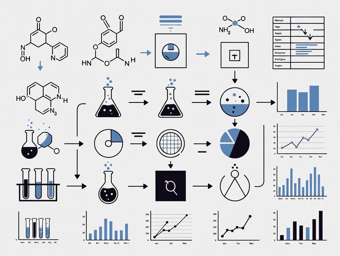
Workflow Visualization
Figure 1: Modified simplex optimization workflow for pharmaceutical development applications. The algorithm iteratively refines experimental conditions until convergence criteria are satisfied.
Figure 2: Geometric transformations in modified simplex optimization. The algorithm reflects the worst vertex (red) away from low-response regions, then expands toward higher-response areas (green).
Applications in Pharmaceutical Development
Analytical Method Optimization
Simplex optimization has demonstrated particular utility in chromatographic method development, where multiple interacting parameters significantly impact separation quality. Applications include:
- HPLC/UPLC method development: Simultaneous optimization of mobile phase composition, gradient profile, temperature, and flow rate [1]
- Capillary electrophoresis: Optimization of buffer pH, concentration, and applied voltage
- Spectroscopic methods: Parameter optimization for atomic absorption and emission techniques
The modified simplex approach typically reduces method development time by 40-60% compared to univariate approaches while producing more robust methods capable of withstanding normal operational variation.
Formulation Development
Pharmaceutical formulation represents an ideal application for simplex optimization due to the complex interactions between multiple components and process parameters. Successful implementations include:
- Solid dosage forms: Optimizing excipient ratios and processing parameters for desired dissolution and stability profiles
- Liquid formulations: Balancing preservative efficacy, viscosity, and stability through component optimization
- Nanoparticle systems: Optimizing multiple characteristics including particle size, polydispersity, and drug loading
Multi-objective simplex approaches enable formulators to balance competing objectives such as maximizing dissolution while minimizing manufacturing cost or stability risks [4].
Process Optimization
Manufacturing process development benefits significantly from simplex methodology through:
- Reaction condition optimization: Simultaneously optimizing yield, purity, and reaction time
- Extraction processes: Maximizing extraction efficiency while minimizing solvent consumption and processing time
- Purification parameters: Optimizing chromatographic separation conditions for biopharmaceutical purification
Table 3: Performance Comparison of Optimization Methods in Pharmaceutical Development
| Optimization Aspect | Univariate (OVAT) | Multivariate Simplex |
|---|---|---|
| Number of Experiments | High (typically 3ⁿ +) | Moderate (typically 10-30) |
| Factor Interactions | Not detectable | Fully characterized |
| Optimal Condition Reliability | Low (may miss true optimum) | High (systematic approach) |
| Resource Consumption | High | Moderate to low |
| Implementation Complexity | Low | Moderate |
| Adaptability to Constraints | Poor | Excellent |
| Multi-Objective Capability | Limited | Strong [4] |
Recent Advances and Future Perspectives
Theoretical understanding of simplex methods has advanced significantly in recent decades. While the simplex method has always demonstrated practical efficiency, theoretical concerns about exponential worst-case performance persisted for decades [3]. Recent work by Huiberts and Bach (2024) has substantially addressed these concerns, providing mathematical justification for the observed efficiency and establishing polynomial-time bounds for simplex performance [3]. These theoretical advances strengthen the foundation for applying simplex methods in regulated pharmaceutical environments.
Future directions for simplex methodology in pharmaceutical research include:
- Hybrid approaches: Integration of simplex methods with other optimization techniques such as genetic algorithms or artificial neural networks
- High-throughput implementation: Automation of simplex optimization using robotic screening systems
- QbD integration: Formal incorporation into Quality by Design frameworks for regulatory submissions
- Multi-scale optimization: Simultaneous optimization of molecular, formulation, and process parameters
The continued development of multi-objective optimization approaches addresses the complex, competing requirements inherent in pharmaceutical development, enabling more systematic and efficient development of robust, high-quality drug products [4].
The simplex is a fundamental geometric concept in multivariate optimization, representing the simplest possible polytope in any given dimension. In the context of optimization algorithms, the simplex provides the foundational geometry for the simplex method, a cornerstone technique for solving linear programming problems. This method operates by navigating the vertices of a polyhedral feasible region defined by constraints, moving from one vertex to an adjacent one to improve the objective function value with each step [5]. The algorithm's name derives from the geometric structure it effectively utilizes, though it operates on simplicial cones rather than simplices themselves [5].
For researchers in drug development, understanding the simplex geometry is crucial for solving complex optimization problems in areas such as formulation development, process optimization, and experimental design. The simplex method provides a systematic approach to finding optimal solutions when multiple constraints—such as resource limitations, chemical compatibilities, or safety thresholds—must be satisfied simultaneously [6].
Geometric Foundation of the Simplex
Mathematical Definition and Properties
A k-simplex is defined as a k-dimensional polytope that represents the convex hull of its k + 1 affinely independent vertices [7]. Formally, given k + 1 points u₀, ..., uₖ in k-dimensional space, the simplex is defined as:
$$ C = \left{ \theta0 u0 + \dots + \thetak uk ~ \Bigg| ~ \sum{i=0}^k \thetai = 1 \text{ and } \theta_i \geq 0 \text{ for } i=0,\dots,k \right} $$
This structure creates the simplest possible convex set in any dimensional space, with the regular simplex exhibiting the highest symmetry properties of any polytope [6]. The simplex method in optimization leverages this geometric structure by traversing the vertices of the constraint polytope, which can be decomposed into simplex elements.
Table: Progression of Regular Simplex Elements Across Dimensions
| Dimension (n) | Simplex Name | Vertices | Edges | Faces | Facets |
|---|---|---|---|---|---|
| 0 | Point | 1 | 0 | 0 | 0 |
| 1 | Line Segment | 2 | 1 | 0 | 0 |
| 2 | Triangle | 3 | 3 | 1 | 3 |
| 3 | Tetrahedron | 4 | 6 | 4 | 4 |
| 4 | 5-cell | 5 | 10 | 10 | 5 |
| 5 | 5-simplex | 6 | 15 | 20 | 6 |
| n | n-simplex | n+1 | n(n+1)/2 | - | n+1 |
The number of m-dimensional faces in an n-simplex is given by the binomial coefficient $\binom{n+1}{m+1}$, demonstrating the combinatorial complexity that arises in higher-dimensional optimization problems [7].
The Standard Simplex in Optimization
The standard simplex or probability simplex is particularly relevant in optimization contexts. This k-dimensional simplex is defined in Rᵏ⁺¹ as:
$$ \left{ \vec{x} \in \mathbf{R}^{k+1} : x0 + \dots + xk = 1, x_i \geq 0 \text{ for } i=0,\dots,k \right} $$
This formulation is essential for problems involving probability distributions, resource allocation, and mixture designs—common scenarios in pharmaceutical development where components must sum to a fixed total (e.g., 100% of a formulation) [7].
The Simplex Algorithm: Movement Through Geometry
Algorithmic Mechanics
The simplex algorithm, developed by George Dantzig in 1947, solves linear programming problems by exploiting the geometry of the feasible region [3] [5]. The fundamental principle stems from the observation that if a linear program has an optimal solution, it must occur at one of the extreme points (vertices) of the polytope defined by the constraints [5].
The algorithm operates through pivot operations that move from one vertex to an adjacent vertex along edges of the polytope, improving the objective function with each move [5]. This movement through the geometric structure continues until no improving adjacent vertex exists, indicating an optimal solution has been found.
Table: Simplex Algorithm Operational Components
| Component | Mathematical Representation | Geometric Interpretation | Role in Optimization |
|---|---|---|---|
| Basic Feasible Solution | Vertex of polytope | Extreme point of feasible region | Starting point for algorithm |
| Pivot Operation | Matrix row operations | Movement to adjacent vertex | Iterative improvement mechanism |
| Reduced Cost | $\bar{c}_D^T$ in tableau | Rate of objective improvement | Optimality condition check |
| Canonical Form | $[1 \ -\bar{c}D^T \ zB]$ | Standardized representation | Computational efficiency |
Movement Mechanisms
The geometry of simplex movement involves several key operations:
Initialization (Phase I): Finding an initial basic feasible solution corresponding to a vertex of the polytope [5].
Optimality Check: Evaluating whether the current vertex is optimal by examining adjacent vertices [5].
Pivot Selection: Choosing a non-basic variable to enter the basis and determining which basic variable must leave, corresponding to selecting which edge to traverse [5].
Termination: Ending the process when no adjacent vertex offers improvement, or identifying an unbounded solution if an infinite edge is encountered [5].
The geometric interpretation reveals why the algorithm is efficient: although the number of vertices grows combinatorially with problem size, the algorithm typically visits only a small fraction of these vertices before finding the optimum [3].
Experimental Protocols for Simplex Optimization
Protocol 1: Standard Simplex Implementation for Formulation Optimization
Purpose: To optimize drug formulation components using the simplex method.
Materials:
- Experimental variables (excipient concentrations)
- Response measurement equipment (dissolution apparatus, HPLC)
- Linear programming software (MATLAB, Python with SciPy, or specialized optimization tools)
Procedure:
Problem Formulation:
- Define objective function (e.g., maximize dissolution rate)
- Identify constraints (e.g., total concentration = 100%, individual component limits)
- Transform to standard form: Maximize $c^Tx$ subject to $Ax \leq b$, $x \geq 0$ [5]
Initialization:
Iteration:
- While reduced costs indicate non-optimality:
- Select entering variable (most negative reduced cost)
- Determine leaving variable via minimum ratio test
- Perform pivot operation to update tableau [5]
- While reduced costs indicate non-optimality:
Termination:
- When all reduced costs are non-negative (maximization problem)
- Extract solution from final tableau
Validation: Confirm optimal solution satisfies all constraints and produces expected improvement in objective function.
Protocol 2: Multi-objective Simplex for Balanced Therapeutic Profile
Purpose: To optimize multiple therapeutic objectives simultaneously using multi-objective simplex approaches.
Materials:
- Conflicting efficacy/toxicity response measures
- Weighting factors for objective importance
- Multi-objective linear programming (MOLP) implementation [4]
Procedure:
Problem Structuring:
- Identify all objective functions (efficacy, stability, manufacturability)
- Establish priority weights or constraint limits for each objective [4]
Simultaneous Optimization:
- Apply modified simplex technique to optimize all objectives concurrently [4]
- Generate Pareto-optimal solutions representing trade-offs
Solution Selection:
- Evaluate efficient solutions based on decision-maker preferences
- Select optimal compromise solution
Advantages: Reduced computational effort compared to sequential optimization; identifies true optimal trade-offs between competing objectives [4].
Visualization of Simplex Algorithm Workflow
The following diagram illustrates the complete workflow of the simplex algorithm in optimization:
The Scientist's Toolkit: Research Reagent Solutions
Table: Essential Computational and Experimental Components for Simplex Optimization
| Research Reagent | Function in Simplex Optimization | Implementation Example |
|---|---|---|
| Linear Programming Solver | Computational engine for simplex algorithm | MATLAB linprog, Python SciPy optimize.linprog, commercial solvers (CPLEX, Gurobi) |
| Sensitivity Analysis Tools | Determines parameter stability and solution robustness | Shadow price calculation, objective coefficient ranging, right-hand-side sensitivity |
| Multi-objective Framework | Extends simplex method to multiple conflicting objectives | Weighted sum method, epsilon-constraint technique, goal programming [4] |
| Tableau Data Structure | Matrix representation of linear program | Two-dimensional array storing coefficients, basic variables, and objective values [5] |
| Constraint Handler | Manages inequality and equality constraints | Slack/surplus variable introduction, artificial variables for Phase I [5] |
| Randomization Module | Improves algorithm performance and avoids worst-case complexity | Random pivot rule implementation, perturbation techniques [3] |
| Visualization Package | Geometric interpretation of algorithm progress | 2D/3D constraint plotting, solution path animation, convergence monitoring |
Advanced Considerations in Simplex Applications
Computational Complexity and Recent Advances
While the simplex method has demonstrated remarkable efficiency in practice since its development by Dantzig, theoretical computer science has revealed concerns about its worst-case complexity. In 1972, mathematicians proved that the time required could grow exponentially with problem size in pathological cases [3].
Recent theoretical breakthroughs have addressed this long-standing issue. Building on landmark work from 2001 by Spielman and Teng that introduced randomness to avoid worst-case scenarios, Bach and Huiberts (2024) have further refined the approach to guarantee significantly lower runtimes [3]. Their work provides stronger mathematical justification for the method's practical efficiency and demonstrates that exponential runtimes do not materialize in practice with appropriate randomization techniques [3].
For drug development researchers, these advances validate reliance on simplex-based optimization in critical development timelines, ensuring predictable computational performance even for large-scale problems involving numerous formulation variables and constraints.
Barycentric Coordinates for Mixture Problems
In pharmaceutical formulation development, barycentric coordinates provide a powerful representation for mixture problems. Any point within a simplex can be expressed as a convex combination of its vertices using barycentric coordinates (v₁, v₂, ..., vₙ) where Σvᵢ = 1 and vᵢ ≥ 0 [6].
This coordinate system naturally represents pharmaceutical formulations where components must sum to 100%, allowing researchers to:
- Systematically explore the entire formulation space
- Identify regions of optimal performance
- Visualize composition-property relationships
- Navigate constraint boundaries effectively
The simplex coordinates provide a pseudo-orthogonal framework that facilitates decomposition of complex mixture relationships, making it particularly valuable for understanding interactions between multiple formulation components [6].
In multivariate optimization, simplex-based methods provide a powerful framework for experimental improvement and process optimization, particularly when detailed mechanistic models of the system are unavailable. These methods are classified into two distinct algorithmic philosophies: the fixed-size basic simplex and the adaptive modified simplex. The fundamental difference lies in their operational dynamics—fixed-size simplex maintains a constant step size throughout the optimization process, while adaptive modified simplex dynamically adjusts its step size and search direction based on landscape feedback [8] [9].
For researchers in drug development, these methods offer systematic approaches to navigate complex experimental spaces where multiple factors simultaneously influence critical outcomes. The basic simplex method, originating from the work of Spendley et al., maintains geometric regularity throughout the optimization process, providing stable but potentially slower convergence [8] [10]. In contrast, the modified simplex approach, most famously implemented in the Nelder-Mead algorithm, introduces adaptive mechanisms that allow the simplex to change shape based on response landscape characteristics, potentially accelerating convergence at the cost of increased complexity [10].
Theoretical Foundations and Algorithmic Mechanisms
Fixed-Size Basic Simplex Methodology
The fixed-size basic simplex operates through a series of predetermined movements, maintaining consistent step sizes throughout the optimization process. This approach uses a regular geometric structure (a simplex) with k+1 vertices for k factors, where each vertex represents a specific combination of factor levels [8]. The algorithm proceeds by reflecting the worst-performing vertex through the centroid of the opposing face, generating new experimental points in a structured manner while maintaining a constant simplex size [9].
Key characteristics of the fixed-size approach include:
- Geometric regularity: The simplex maintains its shape throughout the optimization process
- Fixed step size: Perturbation size remains constant, providing consistent experimental increments
- Systematic reflection: The worst vertex is reflected to generate new experimental conditions
- Boundary handling: Specific rules manage constraints and boundary violations
The basic simplex is particularly valued for its stability and predictable behavior, especially in noisy experimental environments where large, adaptive steps might amplify variability issues [8].
Adaptive Modified Simplex Methodology
The adaptive modified simplex, most prominently implemented in the Nelder-Mead algorithm, introduces flexibility in both step size and direction by allowing the simplex to expand, contract, or reshape itself based on local response characteristics [10]. Unlike its fixed-size counterpart, this approach employs a variable step size mechanism that can accelerate convergence in favorable regions or contract to refine the search in unpromising areas.
The modified simplex incorporates four primary operations:
- Reflection: Projects the worst point through the centroid of the remaining points
- Expansion: Extends further in promising directions when reflection yields significant improvement
- Contraction: Reduces step size when reflection provides moderate improvement
- Shrinkage: Globally reduces simplex size when no improvement is found
A key advancement in modern implementations involves the analytical computation of the reflection parameter (α) rather than relying on fixed heuristic values, enhancing convergence properties [10]. This approach allows the algorithm to make larger steps when progressing toward optima and smaller steps when nearing the optimum region, potentially improving efficiency while maintaining robustness.
Figure 1: Adaptive Modified Simplex Decision Logic
Comparative Performance Analysis
Algorithmic Characteristics and Operational Parameters
Table 1: Fundamental Characteristics of Fixed-Size vs. Adaptive Simplex Methods
| Characteristic | Fixed-Size Basic Simplex | Adaptive Modified Simplex |
|---|---|---|
| Simplex Structure | Regular geometric shape maintained | Shape evolves based on response surface |
| Step Size | Constant throughout optimization | Variable (expands/contracts based on performance) |
| Parameters to Define | Initial step size, reflection coefficient | Reflection, expansion, contraction, shrinkage coefficients |
| Convergence Behavior | Stable, predictable progression | Potentially faster but may oscillate near optima |
| Noise Sensitivity | More robust to experimental noise | More sensitive to noise due to adaptive nature |
| Boundary Handling | Requires explicit constraint management | Can incorporate boundary constraints in operations |
| Computational Complexity | Lower; simple calculations | Higher; multiple operations per iteration |
| Implementation Complexity | Straightforward to implement | More complex decision logic required |
Quantitative Performance Metrics
Table 2: Performance Comparison Under Different Experimental Conditions
| Experimental Condition | Fixed-Size Basic Simplex | Adaptive Modified Simplex |
|---|---|---|
| Low Noise (SNR > 1000) | Slow but reliable convergence | Fast convergence with minimal oscillations |
| High Noise (SNR < 250) | Maintains direction stability | Prone to misdirection; may require restart |
| Low Dimensions (k < 4) | Efficient with minimal overhead | Very efficient with rapid improvement |
| High Dimensions (k > 6) | Computationally expensive | More efficient per evaluation but may require more iterations |
| Factor Step Size (dx) | Critical parameter; optimal ~1-5% of range | Less critical; algorithm adapts step size |
| Computational Resources | Lower memory and processing requirements | Higher memory for storing complex states |
Research comparing these approaches demonstrates that the optimal selection depends heavily on specific experimental conditions. In simulation studies, the adaptive modified simplex generally outperforms the fixed-size approach in low-noise environments and lower-dimensional spaces, while the fixed-size method maintains advantages in high-noise scenarios or when consistent, small perturbations are required to keep processes within specification limits [8].
Experimental Protocols for Pharmaceutical Applications
Protocol 1: Fixed-Size Basic Simplex for Reaction Optimization
Objective: Optimize yield and purity in a synthetic pathway while maintaining temperature and pressure within safe operating boundaries.
Materials and Equipment:
- Reaction vessel with temperature and pressure control
- Analytical HPLC system for purity assessment
- pH meter for monitoring reaction conditions
- Reagents and catalysts as required for synthesis
Experimental Workflow:
Define Optimization Factors and Ranges:
- Factor A: Reaction temperature (30-80°C)
- Factor B: Catalyst concentration (0.1-2.0 mol%)
- Factor C: Reaction time (1-24 hours)
- Factor D: Solvent ratio (0.2-0.8 v/v)
Initialize Simplex:
- Create initial simplex with 5 vertices (k+1 for k=4 factors)
- Set step size to 10% of factor range for each variable
- Define reflection coefficient = 1.0
Iterative Optimization:
- Execute experiments according to current simplex vertices
- Measure responses (yield, purity)
- Calculate composite objective function: 0.6yield + 0.4purity
- Identify worst-performing vertex
- Reflect worst vertex through centroid of remaining vertices
- Verify new vertex stays within constraint boundaries
- If boundary violation occurs, implement projection to feasible region
Termination Criteria:
- Continue until simplex cycles without significant improvement (<2% change in objective function over 3 iterations)
- Maximum of 20 experimental iterations
Data Analysis:
- Plot objective function progression vs. iteration number
- Construct response surfaces based on final simplex vertices
- Identify optimal factor settings from best-performing vertex
Figure 2: Fixed-Size Simplex Experimental Workflow
Protocol 2: Adaptive Modified Simplex for Formulation Development
Objective: Optimize drug formulation composition to maximize dissolution rate while minimizing excipient cost and ensuring stability.
Materials and Equipment:
- Powder blending equipment
- Tablet compression machine
- Dissolution testing apparatus
- Stability chambers (controlled temperature and humidity)
- HPLC system for potency verification
Experimental Workflow:
Define Factors and Objective Function:
- Factor A: API concentration (5-30% w/w)
- Factor B: Binder percentage (1-10% w/w)
- Factor C: Disintegrant percentage (2-15% w/w)
- Factor D: Lubricant percentage (0.5-3% w/w)
- Objective: Maximize Z = 0.5dissolution_rate + 0.3(1/cost) + 0.2*stability_index
Initialize Adaptive Simplex:
- Generate k+1 = 5 initial vertices using Latin Hypercube sampling
- Set initial parameters: α(reflection)=1.0, γ(expansion)=2.0, β(contraction)=0.5, δ(shrinkage)=0.5
Iterative Optimization Cycle:
- Prepare formulations according to current simplex vertices
- Characterize formulations (dissolution, cost calculation, stability testing)
- Rank vertices by objective function value
- Calculate centroid of best k vertices
- Apply reflection operation to generate candidate point
- Evaluate candidate point:
- If best improvement: Apply expansion
- If moderate improvement: Accept reflection
- If slight improvement: Apply contraction
- If no improvement: Apply shrinkage
Convergence Determination:
- Terminate when vertex standard deviation falls below threshold
- Or when simplex volume reduces to predetermined minimum
- Maximum of 15 iterations due to resource constraints
Data Analysis:
- Construct perturbation plots showing factor effects on responses
- Perform robustness analysis around optimal formulation
- Validate optimal formulation with triplicate experiments
Implementation Considerations for Drug Development
The Scientist's Toolkit: Essential Research Reagents and Solutions
Table 3: Key Research Reagents and Solutions for Simplex Optimization Experiments
| Reagent/Solution | Function in Optimization | Application Notes |
|---|---|---|
| pH Buffer Systems | Control and optimize reaction microenvironment | Critical for enzymatic or pH-sensitive synthetic pathways |
| Catalyst Libraries | Screen for optimal reaction acceleration | Vary concentration as factor in synthetic optimization |
| Solvent Mixtures | Modulate polarity and solubility parameters | Adjust ratios as continuous factors in formulation |
| Excipient Blends | Optimize drug delivery characteristics | Varied proportions affect dissolution and stability |
| Stability Indicators | Quantify formulation robustness under stress | Incorporate into objective function for stability |
| Analytical Standards | Quantify yield, purity, and byproducts | Essential for accurate response measurement |
| Mobile Phase Components | HPLC method development and analysis | Can be factors when optimizing analytical methods |
Practical Implementation Guidelines
Successful implementation of simplex methods in pharmaceutical research requires careful consideration of several practical aspects:
Factor Selection and Scaling:
- Select factors with significant expected impact on responses
- Scale factors to similar magnitude (e.g., 0-1 range) to prevent dominance by single variable
- Include both process and composition factors where applicable
Experimental Design Considerations:
- For fixed-size simplex, initial step size should represent practically significant changes
- For adaptive simplex, initial vertices should span feasible region adequately
- Include replication at reference point to estimate experimental error
Response Measurement and Objective Function:
- Incorporate multiple critical quality attributes in objective function
- Apply appropriate weighting to balance competing objectives
- Consider using desirability functions for complex multi-objective optimization
Constraint Management:
- Implement hard constraints for safety-critical parameters
- Use penalty functions for soft constraints in objective function
- Establish boundary violation protocols before beginning experiments
The selection between fixed-size basic simplex and adaptive modified simplex represents a fundamental strategic decision in experimental optimization for pharmaceutical development. The fixed-size approach offers stability and robustness in high-noise environments or when consistent, small perturbations are required to maintain process control. In contrast, the adaptive modified simplex provides accelerated convergence and greater efficiency in well-characterized experimental spaces with lower noise levels.
For drug development applications, the adaptive modified simplex generally offers advantages in early-stage formulation and synthetic route optimization where rapid iteration is valuable and experimental noise can be controlled. The fixed-size approach maintains relevance in manufacturing process optimization and scale-up activities where consistent, controlled adjustments are essential for maintaining quality and regulatory compliance.
Future directions in simplex methodology development include hybrid approaches that combine the stability of fixed-size methods with the efficiency of adaptive approaches, as well as integration with machine learning techniques for initial guidance and anomaly detection [10] [11]. These advances promise to further enhance the utility of simplex methods as essential tools in the pharmaceutical researcher's toolkit.
In the pursuit of efficient and cost-effective drug development, researchers constantly seek superior methods for optimizing complex processes. Within this context, multivariate optimization presents a significant challenge, particularly in early-stage development where resources are limited and experimental data is sparse. The Simplex method emerges as a powerful, sequential optimization technique that enables researchers to navigate multidimensional experimental spaces with remarkable efficiency. Unlike traditional Design of Experiments (DoE) approaches that require extensive upfront experimentation, Simplex methods begin with a minimal set of experiments and then progressively determine the direction toward improved responses through an iterative process of reflection, expansion, and contraction [12]. This paper delineates the specific pharmaceutical use cases where Simplex protocols offer distinct advantages over conventional optimization approaches, providing detailed application notes and experimental protocols for implementation.
Pharmaceutical Applications of Simplex Optimization
Ideal Use Cases and Advantages
Simplex optimization demonstrates particular strength in specific pharmaceutical development scenarios. The table below summarizes the key use cases and the corresponding advantages over traditional methods.
Table 1: Pharmaceutical Use Cases for Simplex Optimization
| Use Case | Key Advantages | Traditional Method Challenge |
|---|---|---|
| Early Bioprocess Development [13] | Rapid identification of optimal conditions with minimal experiments; handles complex, nonlinear data trends | Extensive experimentation required before establishing viable operating windows |
| High-Throughput Chromatography Optimization [13] | Efficiently optimizes multiple response variables (yield, DNA content, HCP) simultaneously; compatible with gridded experimental data | Graphical optimization becomes complex with multiple responses; requires numerous experimental slices |
| Multi-objective Formulation Development | Avoids deterministic weight specification; delivers solutions belonging to Pareto set (non-dominated solutions) [13] | Weight specification requires extensive expert knowledge; solutions may be dominated in all responses |
| Membrane Protein Proteomics [14] | Superior enrichment of hydrophobic and lipidated proteins compared to acetone precipitation | Conventional one-phase extraction methods inefficient for membrane-rich samples |
Simplex in Bioprocess Chromatography
In high-throughput downstream process development, a grid-compatible Simplex variant has demonstrated exceptional performance in optimizing chromatography steps. This approach efficiently manages three critical responses simultaneously: yield, residual host cell DNA content, and host cell protein (HCP) content [13]. The method employs a desirability function to amalgamate these multiple responses into a single objective function, effectively converting a multi-objective problem into a scalar optimization challenge. The Simplex algorithm then navigates the complex space of both experimental conditions and response weights, delivering operating conditions that offer balanced, superior performance across all outputs. This approach has proven successful even with highly nonlinear response surfaces where high-order DoE models struggle [13].
Simplex in Multi-omics Sample Preparation
The SIMPLEX (Simultaneous Metabolite, Protein, Lipid Extraction) protocol represents a specialized liquid-liquid extraction application in analytical pharmacology. This method significantly enriches membrane proteins, transmembrane proteins, and S-palmitoylated proteins from lipid-rich synaptic junctions compared to conventional acetone precipitation [14]. For drug development research focusing on neuronal targets or membrane-bound receptors, this capability is crucial for comprehensive proteomic and phosphoproteomic characterization. The method achieves a 42% enrichment in membrane proteins, enabling more effective mass spectrometry-based identification of challenging hydrophobic protein targets relevant to neurological disorders [14].
Experimental Protocols
Grid-Compatible Simplex for Bioprocess Optimization
Table 2: Reagent Solutions for Bioprocess Optimization
| Research Reagent | Function in Protocol |
|---|---|
| Desirability Function Framework [13] | Amalgamates multiple responses (yield, impurities) into a single objective function |
| Gridded Experimental Space [13] | Pre-processed search space with monotonically increasing integers assigned to factor levels |
| Response Weight Parameters [13] | Incorporated as optimization inputs to avoid deterministic specification |
| Chromatography Resins & Buffers | Experimental materials for which optimal conditions are determined |
Protocol Steps:
- Pre-processing: Convert the gridded experimental search space by assigning monotonically increasing integers to the levels of each process factor (e.g., pH, conductivity, buffer concentration). Replace any missing data points with highly unfavorable surrogate values to guide the algorithm away from these regions [13].
- Initial Simplex Formation: Define a starting point or initial simplex within the processed experimental space. The number of vertices in this simplex equals n+1, where n is the number of variables being optimized [12] [15].
- Iterative Optimization:
- Evaluation: Conduct experiments at the conditions defined by the simplex vertices and measure all relevant responses (yield, DNA, HCP).
- Desirability Calculation: Apply the desirability approach to merge multiple responses into a total desirability value (D). Use Equations 1 and 2 for maximizing (e.g., yield) and minimizing (e.g., impurities) responses respectively, and Equation 3 to calculate the composite D [13].
- Simplex Transformation: Based on the response values, apply Simplex rules (reflection, expansion, contraction) to determine the coordinates of the next experimental point, moving away from unfavorable conditions and toward promising regions [12] [13].
- Termination: Continue iterations until the method identifies an optimum (no further improvement in D is observed) or meets predefined convergence criteria [13].
SIMPLEX Extraction for Membrane Proteomics
Table 3: Reagent Solutions for Membrane Proteomics
| Research Reagent | Function in Protocol |
|---|---|
| Methyl-tert-butylether (MTBE) [14] | Organic solvent for lipid extraction and membrane solubilization |
| Methanol [14] | Homogenization agent and protein precipitant |
| Triethylammonium bicarbonate (TEAB) [14] | Buffering agent for maintaining pH during protein digestion |
| Trypsin (Mass Spectrometry Grade) [14] | Proteolytic enzyme for protein digestion into analyzable peptides |
| Tris(2-carboxyethyl)phosphine (TCEP) [14] | Reducing agent for breaking protein disulfide bonds |
| Iodoacetamide (IAA) [14] | Alkylating agent for cysteine side chain modification |
Protocol Steps:
- Homogenization: Resuspend the membrane-enriched sample (e.g., synaptic junctions) in 225 µL of methanol. Perform three freeze-thaw cycles with intermediate ultrasonication to thoroughly homogenize the sample [14].
- Lipid Extraction: Add 750 µL of MTBE to the homogenate and incubate for 1 hour at 950 rpm and 4°C to solubilize membranes and extract lipids [14].
- Phase Separation: Add 188 µL of dd water to induce phase separation. Centrifuge at 10,000 × g for 10 minutes at 4°C. Remove and discard the upper organic phase containing lipids [14].
- Protein Precipitation: To the remaining lower phase, add 527 µL of methanol and incubate at -20°C for 2 hours to precipitate proteins. Pellet proteins by centrifuging at 13,500 × g for 30 minutes [14].
- Protein Digestion: Resuspend the protein pellet in 8 M urea, 0.1% rapigest in 50 mM TEAB buffer. Reduce proteins with 10 mM TCEP (1 hour, 22°C) and alkylate with 40 mM IAA (30 minutes, room temperature in the dark). Dilute with TEAB to reduce urea concentration below 1 M, then digest with trypsin (enzyme-to-substrate ratio 1:40 w/w) for 16 hours at 37°C [14].
- Analysis: Terminate digestion with formic acid, centrifuge, and desalt the peptides using C18 solid-phase extraction before LC-MS/MS analysis [14].
Workflow Visualization
The following diagram illustrates the logical workflow and decision process for implementing the grid-compatible Simplex method in pharmaceutical development:
Diagram 1: Simplex Optimization Workflow
The strategic implementation of Simplex methods addresses critical inefficiencies in pharmaceutical development, particularly for early-stage process optimization, multi-objective formulation challenges, and specialized analytical preparations. The grid-compatible Simplex algorithm provides a robust framework for navigating complex experimental spaces with minimal experimental runs, while the SIMPLEX extraction protocol offers a superior technical approach for enriching challenging membrane protein targets. By integrating these protocols into their multivariate optimization strategies, researchers and drug development professionals can accelerate development timelines, improve resource utilization, and gain deeper insights into complex biological systems relevant to therapeutic development.
Implementing the Simplex Protocol: A Step-by-Step Guide for Drug Development
The Simplex Method is a foundational algorithm in linear programming and a critical component in multivariate optimization protocol research. It operates by systematically moving from one corner point (extreme point) of the feasible solution space, defined by the problem's constraints, to an adjacent one, improving the objective function value with each step until the optimal solution is found [5]. This method is particularly valued for solving complex resource allocation problems prevalent in pharmaceutical development, such as optimizing reaction conditions, resource scheduling, and raw material blending under multiple constraints.
In the context of modern optimization research, the Simplex Method maintains its relevance even with the development of alternative approaches like Interior Point Methods (IPMs). While IPMs offer polynomial-time complexity and can be exceptionally powerful for very large-scale problems, the Simplex Method often demonstrates superior performance for many practical problems and remains heavily utilized in operational research contexts, including decomposition techniques and column generation schemes [16]. Its geometrical intuition and iterative improvement process make it particularly accessible for researchers modeling complex multivariate systems.
Theoretical Foundation: From LP Formulation to Initial Simplex
Standard Form Conversion
The algorithm requires the linear programming model to be in standard equation form with non-negative right-hand sides and variables [17]. The conversion process involves:
- Slack Variables: Convert ≤ inequalities into equations by adding non-negative slack variables. For example: ( x2 + 2x3 \leq 3 ) becomes ( x2 + 2x3 + s1 = 3 ) with ( s1 \geq 0 ) [5].
- Surplus Variables: Convert ≥ inequalities into equations by subtracting non-negative surplus variables.
- Unrestricted Variables: Replace free variables with the difference of two non-negative variables.
The resulting system forms ( A\mathbf{x} = \mathbf{b} ) with ( \mathbf{x} \geq \mathbf{0} ), where ( A ) is an ( m \times n ) matrix with full row rank [5].
Mathematical Representation
The algorithm utilizes a simplex tableau to organize computations [5]. The initial tableau structure is:
[ \begin{bmatrix} 1 & -\mathbf{c}^T & 0 \ 0 & \mathbf{A} & \mathbf{b} \end{bmatrix} ]
Where ( \mathbf{c} ) represents the objective function coefficients, ( \mathbf{A} ) is the coefficient matrix of constraints, and ( \mathbf{b} ) is the right-hand side vector. Through pivot operations, the tableau is transformed into canonical form, revealing basic feasible solutions and their corresponding objective values.
Table 1: Key Components of the Initial Simplex Tableau
| Component | Symbol | Description | Role in Optimization |
|---|---|---|---|
| Decision Variables | ( x_j ) | Variables representing quantities to be determined | Fundamental units of the solution space |
| Objective Coefficients | ( c_j ) | Coefficients of variables in the objective function | Determine direction of optimization improvement |
| Constraint Matrix | ( A ) | Coefficients of constraints in equation form | Defines the feasible region geometry |
| Right-Hand Side | ( b ) | Constants in constraint equations | Sets capacity limits for resources |
| Slack/Surplus Variables | ( s_i ) | Added variables to convert inequalities to equations | Transform constraint representation |
Experimental Protocol: Constructing the Initial Simplex
Phase I: Initialization and Basic Feasible Solution
The process of finding an initial basic feasible solution constitutes Phase I of the simplex algorithm [5]:
- Problem Formulation: Clearly define the objective function and all constraints based on the optimization problem.
- Standard Form Conversion: Introduce slack, surplus, and artificial variables as needed to transform all constraints into equations.
- Initial Tableau Construction: Set up the initial simplex tableau with the objective function last.
- Artificial Objective Function: For problems requiring artificial variables, create a Phase I objective function that minimizes the sum of artificial variables.
- Feasibility Check: Apply pivot operations until all artificial variables are driven from the basis (or their sum is minimized to zero), indicating a feasible solution has been found.
The outcome of Phase I is either a basic feasible solution to begin Phase II optimization or the determination that the feasible region is empty (infeasible problem) [5].
Workflow Visualization
The following diagram illustrates the complete experimental workflow from problem formulation to optimal solution:
Research Reagent Solutions: Computational Tools for Simplex Implementation
Successful implementation of the simplex protocol requires specific computational tools and analytical approaches:
Table 2: Essential Research Reagents for Simplex Protocol Implementation
| Reagent Category | Specific Tools | Function in Protocol |
|---|---|---|
| Computational Environment | MATLAB, Python with NumPy/SciPy, R | Matrix manipulation for tableau operations and pivot selection |
| Optimization Libraries | Google OR-Tools, IBM CPLEX, SciPy Optimize | Provide pre-implemented simplex variants for validation |
| Visualization Tools | Graphviz DOT language, matplotlib, plotly | Create workflow diagrams and solution space representations |
| Linear Algebra Systems | LU decomposition routines, matrix inversion algorithms | Efficiently handle pivot operations and basis updates |
| Constraint Processors | Symbolic math toolkits, automatic differentiation | Convert inequality constraints to standard form equations |
Advanced Applications: Modified Simplex for Complex Optimization Scenarios
Multi-Criteria Optimization in Fuzzy Environments
Recent research has extended the simplex method to handle multi-criteria optimization problems under uncertainty, particularly valuable for pharmaceutical development where criteria may be contradictory or immeasurable [18]. The modified approach integrates fuzzy set theory with the simplex framework:
- Fuzzy Criteria Evaluation: Decision makers provide fuzzy assessments of immeasurable criteria using linguistic variables.
- Simplex Modification: The traditional simplex method is adapted to process these fuzzy evaluations alongside measurable criteria.
- Pareto Optimal Solutions: The algorithm identifies compromise solutions that balance multiple conflicting objectives.
- Convergence Assurance: A theorem guarantees the solution sequence converges to the minimum criteria values [18].
This hybrid approach has demonstrated practical utility in real-world applications such as optimizing benzene production processes [18].
Computational Mechanics of Pivot Operations
The geometrical movement between corner points is implemented computationally through pivot operations:
Table 3: Pivot Operation Decision Parameters
| Decision Point | Calculation Method | Stopping Condition | ||
|---|---|---|---|---|
| Entering Variable | Max absolute negative reduced cost: ( \max_j | \bar{c}_j < 0 | ) | All reduced costs ≥ 0 |
| Leaving Variable | Minimum ratio test: ( \mini { bi/a{ij} | a{ij} > 0 } ) | All ratios negative (unbounded) | ||
| Pivot Element | Intersection of entering column and leaving row | Matrix singularity check | ||
| Optimality Check | All reduced costs non-negative | Optimal solution found |
Application Notes for Pharmaceutical Research
Protocol Implementation Guidelines
When applying the simplex method to drug development optimization:
- Constraint Modeling: Accurately model production constraints as linear inequalities, considering reaction times, resource availability, and purity requirements.
- Objective Specification: Clearly define the optimization target (cost minimization, yield maximization) with appropriate coefficients.
- Sensitivity Analysis: Conduct post-optimality analysis to determine how changes in constraint parameters affect the optimal solution.
- Validation: Verify results through multiple simplex implementations or alternative optimization approaches where feasible.
Integration with Broader Optimization Framework
The simplex method serves as a fundamental component within a comprehensive multivariate optimization protocol. Its strengths in providing exact solutions to linear problems complement other optimization approaches:
- Decomposition Schemes: The simplex method can be effectively combined with column generation techniques for discrete optimization problems like optimal transport [16].
- Hybrid Approaches: For non-linear or fuzzy optimization scenarios, modified simplex procedures can be integrated with fuzzy mathematics and other optimality principles [18].
- Benchmarking: Use simplex solutions as benchmarks for evaluating heuristic or metaheuristic approaches to complex scheduling problems in pharmaceutical manufacturing [19].
This primer establishes the foundational framework for constructing initial simplex configurations within multivariate optimization research, providing researchers with practical protocols for implementation across diverse pharmaceutical development scenarios.
Core Mathematical Operations of the Simplex Protocol
The Nelder-Mead simplex method is a cornerstone of derivative-free multivariate optimization, relying on a geometric structure called a simplex—an n-dimensional polytope defined by n+1 vertices [20]. The algorithm iteratively improves this simplex through a series of geometric operations, navigating the parameter space without requiring gradient information [21]. These operations form the fundamental "iterative engine" that enables the protocol to converge toward optimal solutions, making it particularly valuable for complex optimization landscapes in scientific and engineering disciplines.
Reflection Operation Protocol
The reflection operation generates a new trial point by moving away from the worst-performing vertex of the simplex, under the assumption that a better point lies in the opposite direction.
Mathematical Formulation: Let ( Xh ) be the vertex with the highest (worst) objective function value, and let ( M ) be the centroid of the remaining vertices (excluding ( Xh )). The reflected point ( Xr ) is calculated as [22]: [ Xr = M + \alpha(M - X_h) ] where ( \alpha ) is the reflection coefficient, typically set to 1 [20]. This operation preserves the volume of the simplex while exploring promising directions away from poor regions of the parameter space.
Experimental Protocol:
- Vertex Evaluation: Calculate objective function values ( f(Xi) ) for all vertices ( X1, X2, ..., X{n+1} )
- Identify Worst Vertex: Determine ( Xh ) where ( f(Xh) = \max{f(X1), f(X2), ..., f(X_{n+1})} )
- Compute Centroid: Calculate ( M = \frac{1}{n} \sum{i \neq h} Xi )
- Generate Reflection: Compute ( Xr = M + \alpha(M - Xh) )
- Evaluate Reflection: Calculate ( f(X_r) ) for comparison
Expansion Operation Protocol
The expansion operation extends the reflection further when the reflected point shows significant improvement, enabling more aggressive exploration of promising regions.
Mathematical Formulation: If the reflected point ( Xr ) represents sufficient improvement (( f(Xr) < f(Xl) ) where ( Xl ) is the best vertex), an expansion point ( Xe ) is generated [20] [22]: [ Xe = M + \gamma(X_r - M) ] where ( \gamma ) is the expansion coefficient, typically set to 2 [20]. This operation increases the simplex volume to accelerate progress toward optima.
Decision Protocol:
- Evaluate Reflection: Compare ( f(Xr) ) with current best value ( f(Xl) )
- Expansion Condition: If ( f(Xr) < f(Xl) ), proceed with expansion
- Generate Expansion: Compute ( Xe = M + \gamma(Xr - M) )
- Evaluate Expansion: Calculate ( f(X_e) )
- Selection: Replace ( Xh ) with the better of ( Xr ) and ( X_e )
Contraction Operation Protocol
Contraction operations reduce the simplex size when reflection fails to produce improvement, enabling finer search resolution and adaptation to complex response surfaces.
Matraction Formulation: Two contraction variants exist based on reflection performance [20]:
Outside Contraction (when ( f(Xr) ) is better than ( Xh ) but not the best): [ Xc = M + \beta(Xr - M) ] where ( \beta ) is the contraction coefficient, typically 0.5 [20]
Inside Contraction (when ( f(Xr) ) is worse than ( Xh )): [ Xc = M - \beta(M - Xh) ]
Experimental Protocol:
- Performance Assessment: Compare ( f(X_r) ) with all vertex values
- Contraction Type Selection: Choose outside or inside contraction based on relative performance
- Generate Contraction Point: Compute ( X_c ) using appropriate formula
- Evaluate Contraction: Calculate ( f(X_c) )
- Replacement Decision: Replace ( Xh ) with ( Xc ) if improvement occurs; otherwise, proceed to shrinkage
Quantitative Performance Analysis
Operational Efficiency Across Problem Domains
Table 1: Simplex Operation Efficiency in Noisy Optimization Problems [21]
| Operation Type | Success Rate (%) | Average Improvement per Step | Distortion in Simplex Size (DSS) | Application Context |
|---|---|---|---|---|
| Reflection | 68.4 | 24.7% | 1.02 | Standard landscape exploration |
| Expansion | 71.9 | 31.2% | 1.87 | Aggressive progression toward optima |
| Contraction | 63.1 | 18.5% | 0.53 | Resolution refinement |
| Shrinkage | 42.7 | -5.3% | 0.38 | Recovery from stagnation |
The adaptive Nelder-Mead algorithm (ANMA) demonstrates superior performance in noisy optimization landscapes compared to the standard implementation (SNMA). In complex nonlinear least-squares problems with experimental noise, ANMA achieved approximately 35% higher convergence probability and 28% faster parameter resolution by adaptively adjusting simplex operations based on landscape characteristics [21].
Parameter Configuration Guidelines
Table 2: Optimal Parameter Settings for Pharmaceutical Applications
| Parameter | Standard Value | Adaptive Range | Problem Sensitivity | Effect on Convergence |
|---|---|---|---|---|
| Reflection (α) | 1.0 | 0.8-1.2 | Low | Governs exploration breadth |
| Expansion (γ) | 2.0 | 1.5-3.0 | High | Controls aggressive progression |
| Contraction (β) | 0.5 | 0.3-0.7 | Medium | Determines refinement resolution |
| Shrinkage (δ) | 0.5 | 0.4-0.6 | Low | Recovery from complex landscapes |
Pharmaceutical Application Protocol
Drug Formulation Optimization Workflow
The simplex protocol enables efficient optimization of pharmaceutical formulations where multiple conflicting objectives must be balanced, such as bioavailability, stability, and production cost [23].
Experimental Protocol:
- Parameter Space Definition:
- Identify critical formulation parameters (excipient ratios, processing variables)
- Establish feasible ranges based on physicochemical constraints
- Define objective function incorporating multiple performance metrics
Initial Simplex Design:
- Generate n+1 formulations using systematic experimental design
- Ensure non-degenerate simplex geometry
- Incorporate formulation expertise in initial vertex selection
Iterative Optimization Cycle:
- Prepare and characterize formulations corresponding to simplex vertices
- Evaluate objective function (e.g., dissolution profile, stability metrics)
- Apply reflection, expansion, or contraction operations based on performance
- Continue until convergence criteria satisfied
Multi-Objective Optimization in Drug Development
Pharmaceutical development inherently involves multiple competing objectives, requiring specialized approaches to balance efficacy, safety, and manufacturability [18] [23].
Pareto Optimization Protocol:
- Objective Function Definition:
- Transform each critical quality attribute to normalized deviation from target
- Apply weighting factors based on therapeutic priority
- Construct aggregate objective function: [ cost = \frac{\sum wi \cdot |fi - f{i, target}| / f{i, target}}{\sum w_i} ]
Fuzzy Optimization Framework:
- Incorporate expert knowledge through fuzzy evaluation of immeasurable criteria
- Apply hybrid maximin and Pareto optimality principles [18]
- Handle uncertainty in biological response measurements
Decision Support Implementation:
- Present Pareto-optimal solutions to development team
- Enable interactive exploration of formulation trade-offs
- Incorporate regulatory constraints throughout optimization process
Research Reagent Solutions
Table 3: Essential Computational Tools for Simplex Optimization Research
| Research Tool | Function | Application Context | Implementation Example |
|---|---|---|---|
| Adaptive NMA (ANMA) | Dynamic parameter adjustment | Noisy experimental data | Pharmaceutical formulation optimization [21] |
| Multi-Objective NBI | Pareto front generation | Conflicting objectives | Drug property balancing [24] |
| Fuzzy Evaluation | Immeasurable criteria handling | Expert knowledge integration | Biological response optimization [18] |
| Factor Analysis | Response correlation modeling | Multivariate optimization | Quality by Design (QbD) implementation [24] |
| Robust Cost Function | Weighted objective combination | Priority-based optimization | Formulation parameter tuning [25] |
Convergence and Termination Criteria
Effective implementation requires precise convergence monitoring to balance computational efficiency with solution quality.
Termination Protocol:
- Standard Deviation Criterion: Terminate when standard deviation between simplex vertices falls below threshold (e.g., 1×10⁻⁴) [20]
- Simplex Size Monitoring: Track distortion in simplex size (DSS) throughout iterative process [21]
- Performance Stagnation: Monitor improvement rate across iterations
- Iteration Limit: Implement maximum iteration count as fallback (e.g., 1000 iterations) [20]
Conformance Verification:
- Validate solution robustness through perturbation analysis
- Confirm physiological relevance of optimized parameters
- Verify manufacturability within design space boundaries
The iterative engine of reflection, expansion, and contraction operations provides a robust foundation for multivariate optimization in pharmaceutical development. By adapting these core operations to specific research contexts and implementing rigorous experimental protocols, researchers can efficiently navigate complex design spaces to identify optimal formulations balancing multiple critical quality attributes.
In drug discovery and analytical chemistry, developers routinely face the challenge of optimizing multiple, often conflicting, objectives simultaneously. A formulation scientist might need to maximize product purity while minimizing production cost and processing time. Such multi-objective optimization problems are characterized by vast, complex solution spaces where improving one objective often leads to the deterioration of another [26]. Traditional single-variable (univariate) optimization approaches are inadequate for these scenarios as they optimize conditions one-by-one while holding others constant, failing to capture critical interaction effects between variables and potentially missing the true optimal conditions [27].
The integration of the desirability function with robust optimization algorithms provides a powerful framework for confronting these challenges. This approach allows researchers to transform multiple responses into a single, dimensionless metric that can be systematically optimized. Within this framework, the simplex method serves as a particularly effective optimization engine, especially when dealing with complex experimental landscapes where mathematical derivatives are unobtainable or when processes are characterized by uncertainty and fuzzy criteria [27] [18]. This protocol details the application of this combined approach, providing a structured methodology for researchers in drug development and related fields.
Theoretical Foundation
The Desirability Function
The desirability function, introduced by Derringer and Suich, is a mathematical tool for converting multiple response variables into a single, comprehensive metric. Its core principle involves transforming each individual response ( yi ) into a partial desirability function ( di ), which ranges from 0 (completely undesirable) to 1 (fully desirable). The form of ( d_i ) depends on the optimization goal for that particular response:
For "Higher is Better" (Maximization): ( di = \begin{cases} 0 & \text{if } yi < L \ \left( \frac{yi - L}{T - L} \right)^s & \text{if } L \leq yi \leq T \ 1 & \text{if } y_i > T \end{cases} ) where ( L ) is the lower specification limit, ( T ) is the target value (often the maximum practical value), and ( s ) is a user-defined weight.
For "Lower is Better" (Minimization): ( di = \begin{cases} 1 & \text{if } yi < T \ \left( \frac{U - yi}{U - T} \right)^s & \text{if } T \leq yi \leq U \ 0 & \text{if } y_i > U \end{cases} ) where ( U ) is the upper specification limit and ( T ) is the target.
For "Target is Best": ( di = \begin{cases} \left( \frac{yi - L}{T - L} \right)^s & \text{if } L \leq yi \leq T \ \left( \frac{U - yi}{U - T} \right)^t & \text{if } T \leq y_i \leq U \ 0 & \text{otherwise} \end{cases} ) where ( s ) and ( t ) are weights shaping the function around the target ( T ).
These individual desirabilities are then combined into an overall desirability index, ( D ), using the geometric mean: ( D = (d1 \times d2 \times \cdots \times d_n)^{1/n} ) This overall desirability ( D ) becomes the single objective function for the optimization algorithm. A value of ( D=1 ) represents the ideal case where all responses are on target, while ( D=0 ) indicates that at least one response is outside its acceptable limits [27].
The Simplex Method of Optimization
The simplex method used in experimental optimization (distinct from the Dantzig simplex method for linear programming) is a sequential search technique that does not require the calculation of derivatives. It is therefore classified as a direct search method and is particularly valuable when the functional relationship between variables and the response is complex or unknown [27].
The method operates using a geometric figure called a simplex. For ( n ) factors to optimize, the simplex is defined by ( n+1 ) points in the factor space. For example, with two factors, the simplex is a triangle. The core algorithm, the Nelder-Mead simplex, proceeds by iteratively reflecting, expanding, or contracting the simplex away from the point with the worst performance, thus "rolling" itself towards an optimum [27]. This makes it highly effective for navigating response surfaces with potential interactions between variables, a task where univariate methods fail.
Synergistic Integration in a Multi-Objective Context
The power of this approach lies in the synergy between its components. The desirability function translates a complex, multi-criteria problem into a single, quantifiable objective: maximize ( D ). The simplex algorithm then efficiently solves this problem by navigating the factor space, dynamically adjusting the experimental conditions based on the observed ( D ) values without needing to know the underlying mathematical model of each response. This hybrid approach is highly effective for solving Multi-objective Linear Programming (MOLP) problems and has demonstrated reduced computational effort compared to other techniques like preemptive goal programming [4] [18]. Furthermore, the framework can be extended to handle fuzzy environments, where criteria or constraints are not crisp but are described by linguistic variables, allowing the incorporation of expert knowledge and experience from decision-makers [18].
Application Notes & Protocols
Protocol: Multi-Objective Optimization of an HPLC Method for Drug Analysis
This protocol outlines the steps for optimizing a High-Performance Liquid Chromatography (HPLC) method for quantifying an active pharmaceutical ingredient (API), such as Losartan Potassium, using a desirability-simplex approach [28]. The goal is to simultaneously achieve optimal resolution, analysis time, and peak symmetry.
1. Problem Definition and Goal Setting
- Objective: Develop a robust HPLC method to quantify Losartan Potassium in capsules.
- Critical Responses (Objectives):
- ( y1 ): Resolution (Rs) from closest impurity. Goal: Maximize (Target ≥ 2.0).
- ( y2 ): Analysis time (t). Goal: Minimize (Target ≤ 10 min).
- ( y_3 ): Peak Asymmetry Factor (As). Goal: Target is 1.0.
- Critical Factors (Variables):
- ( x1 ): pH of the mobile phase buffer.
- ( x2 ): Concentration of the organic modifier (e.g., Acetonitrile %).
- ( x3 ): Flow rate (mL/min).
- ( x4 ): Column temperature (°C).
2. Experimental Design and Initial Simplex
- Define the feasible range for each factor based on preliminary experiments or literature.
- Construct an initial simplex in the 4-dimensional factor space. This requires 5 initial experimental runs (n+1, where n=4). These initial points can be selected using a preliminary fractional factorial design to efficiently scout the design space [28].
3. Defining the Desirability Functions For each experimental run, the responses are measured and converted into partial desirabilities. Table 1: Specification of Partial Desirability Functions for HPLC Optimization
| Response Variable | Goal | Lower Limit (L) | Target (T) | Upper Limit (U) | Weights (s, t) |
|---|---|---|---|---|---|
| Resolution (Rs) | Maximize | 1.5 | 2.0 | - | 1 |
| Analysis Time (t) | Minimize | - | 5.0 | 10.0 | 1 |
| Peak Asymmetry (As) | Target | 0.8 | 1.0 | 1.2 | 1, 1 |
4. Sequential Simplex Optimization The following workflow outlines the iterative optimization process.
Diagram 1: Workflow for Simplex-Desirability Optimization. The process iterates until the change in the overall desirability (D) between iterations falls below a pre-defined threshold.
- Iteration: For the initial simplex, run all 5 experiments and calculate ( D ). Identify the experiment with the lowest ( D ) (worst vertex).
- Reflection: Generate a new vertex by reflecting the worst vertex through the centroid of the remaining points.
- Decision: Run the experiment at the new reflected vertex and calculate its ( D ).
- If the new ( D ) is better than the second-worst, keep it.
- If it is the best so far, try an expansion to move further in that direction.
- If it is worse, perform a contraction to find a better point closer to the centroid.
- Termination: The algorithm terminates when the change in ( D ) falls below a pre-specified threshold or the simplex shrinks below a certain size, indicating convergence [27].
5. Validation Once the optimal conditions are identified (e.g., Potassium Phosphate Buffer pH 6.2, 35% Acetonitrile, Flow Rate 1.0 mL/min, Column Temperature 35°C [28]), a final validation experiment is performed. The method should be validated according to ICH guidelines, assessing accuracy, precision, selectivity, robustness, and linearity.
The Scientist's Toolkit: Research Reagent Solutions
Table 2: Essential Materials for Multivariate HPLC Optimization
| Item | Function / Role in Optimization |
|---|---|
| HPLC System with DAD/UV Detector | Enables precise pumping of mobile phase, sample injection, separation on the column, and detection of analytes. Critical for measuring response variables (retention time, peak area, etc.). |
| C8 or C18 Analytical Column | The stationary phase where chromatographic separation occurs. Its properties (length, particle size, ligand) are key factors in the optimization. |
| Buffer Salts (e.g., K₂HPO₄/KH₂PO₄) | Used to prepare the aqueous component of the mobile phase. Buffer pH and concentration are often critical optimized factors affecting ionization and selectivity. |
| Organic Modifiers (e.g., Acetonitrile, Methanol) | The organic component of the mobile phase. Its concentration is a primary factor for controlling retention time and resolution. |
| Analytical Standard of the API | High-purity reference material required to prepare calibration standards and accurately measure method performance responses. |
| Experimental Design & Data Analysis Software | Software (e.g., JMP, Design-Expert, MATLAB ) is essential for designing the initial experiments, calculating the simplex, and modeling the desirability function. |
Advanced Application: Optimization in a Fuzzy Environment
Many real-world technological processes are characterized by uncertainty, including immeasurable or linguistically described criteria (e.g., "good crystal habit" or "ease of filtration"). For such problems, the simplex-desirability framework can be modified to work in a fuzzy environment [18].
The methodology involves using fuzzy set theory to define desirability functions. Instead of crisp limits, membership functions define the partial desirability ( \tilde{d_i} ). The overall desirability ( \tilde{D} ) becomes a fuzzy index, and the optimization can incorporate principles like Pareto optimality and maximin to find the best compromise solution. This often requires the involvement of a Decision Maker (DM)—a subject matter expert—to fuzzily evaluate criteria that cannot be physically measured [18].
Diagram 2: Fuzzy Simplex-Desirability Logic. This approach integrates expert knowledge for problems with qualitative or uncertain objectives.
The integration of the desirability function with the simplex optimization protocol provides a structured and powerful strategy for conquering complex multi-objective problems in drug design and analytical science. This approach enables the systematic balancing of conflicting goals, such as maximizing efficacy while minimizing toxicity and cost, through a mechanism that is both computationally efficient and intuitively accessible to scientists. By transforming a multi-faceted problem into a single, quantifiable metric of "desirability," and then employing a robust direct search algorithm to maximize it, researchers can navigate complex experimental landscapes more effectively than with traditional univariate methods. The flexibility of this framework, including its extension into fuzzy optimization for handling uncertainty and qualitative criteria, makes it an indispensable tool for modern research and development, ensuring that the final solution represents a scientifically sound and practically viable compromise across all critical objectives.
Impurity profiling is a critical analytical activity within pharmaceutical development and manufacturing, determining the chemical purity, quality, and safety of drug products. It involves the identification and quantification of all components coexisting with an Active Pharmaceutical Ingredient (API), including residual solvents, degradation products, and process-related contaminants. The presence of such impurities can significantly impact a product's efficacy, stability, and safety, making their rigorous detection and control a non-negotiable aspect of quality assurance [29].
Chromatographic techniques, notably High-Performance Liquid Chromatography (HPLC) and Ultra-High-Performance Liquid Chromatography (UPLC), have emerged as the cornerstone of modern impurity profiling due to their superior separation efficiency and reliability. However, traditional method development, often employing a One-Factor-at-a-Time (OFAT) approach, can lead to suboptimal separation, particularly for complex mixtures of an API and its numerous impurities [30]. This case study details the application of a systematic multivariate optimization simplex protocol to develop a robust, precise, and accurate UPLC method for the simultaneous determination of the antiretroviral drug Darunavir and its seventeen related impurities. This work is framed within a broader research thesis on advanced optimization protocols, demonstrating how structured, multi-objective computational techniques can overcome the limitations of conventional empirical methods in analytical chemistry [4].
Theoretical Framework: Simplex-Based Multi-Objective Optimization
The optimization in this case study is grounded in the principles of Multi-Objective Linear Programming (MOLP) solved via a simplex technique. In the context of chromatographic method development, this translates to a scenario where multiple Critical Method Attributes (CMAs)—such as resolution between peak pairs, peak tailing, and total runtime—must be optimized simultaneously. Often, these objectives conflict; for instance, improving resolution might require a slower gradient, thereby increasing analysis time [4].
The simplex-based multi-objective optimization approach provides a computational framework to navigate these trade-offs efficiently. Unlike goal programming or other techniques, the devised simplex technique optimizes all objectives concurrently within the defined experimental domain, significantly reducing computational effort while yielding a set of efficient, Pareto-optimal solutions. A solution is considered Pareto-optimal if no objective can be improved without worsening another. For the chromatographer, this means identifying the method conditions that deliver the best possible compromise between all desired separation criteria [4].
Experimental Design and Workflow
The method development followed the Analytical Quality by Design (AQbD) framework, which emphasizes a systematic, science-based approach for enhancing method robustness and reliability. The workflow, illustrated below, integrates the AQbD paradigm with the simplex optimization protocol [30].
Define the Analytical Target Profile (ATP) and Critical Method Attributes (CMAs)
The first step in AQbD is to define the Analytical Target Profile (ATP), which outlines the required quality characteristics of the analytical method. For this study, the ATP was defined as a chromatographic method capable of delivering optimal resolution between Darunavir and its seventeen impurities, while also achieving symmetrical peak shapes [30].
From this ATP, the following Critical Method Attributes (CMAs) were derived as the key performance metrics to be optimized:
- Rs_min: The resolution of the least-resolved critical peak pair.
- N_peaks: The total number of impurities resolved from the main peak.
- Tailing Factor (Tf): The peak symmetry for the Darunavir peak.
Identify Critical Method Variables (CMVs)
Critical Method Variables (CMVs) are the instrumental and chemical parameters that significantly influence the CMAs. Based on prior knowledge and initial screening, the following CMVs were selected for optimization:
- pH of the aqueous mobile phase buffer.
- Gradient Time (t_G): The time for the organic modifier to increase from initial to final concentration.
- Column Temperature (T_col).
- Concentration of the Buffer (C_buf).
Implementation of the Simplex Optimization Protocol
The multi-objective simplex protocol was applied to navigate the complex, multi-dimensional factor space defined by the CMVs. The algorithm proceeds as follows [4]:
- Initialization: An initial simplex is created with a number of vertices equal to n+1, where
nis the number of CMVs being optimized. - Evaluation: Each vertex of the simplex represents a specific combination of CMV values. The chromatographic method for each vertex is run, and the resulting CMAs (Rsmin, Npeaks, Tf) are measured.
- Comparison and Iteration: The vertex (method condition) yielding the worst composite performance is identified and reflected through the centroid of the opposite face of the simplex, generating a new vertex.
- Convergence: This process of reflection, expansion, and contraction continues iteratively until the simplex converges on an optimum where further improvements to all CMAs are no longer possible, representing the Pareto-optimal solution.
Results and Discussion
Optimized Chromatographic Conditions
The application of the simplex optimization protocol yielded a set of robust chromatographic conditions that successfully met the ATP, as detailed in the table below.
Table 1: Final Optimized Chromatographic Conditions
| Parameter | Optimized Condition |
|---|---|
| Analytical Technique | UPLC with PDA and MS Detection |
| Column | BEH C18 (100 mm x 2.1 mm, 1.7 µm) |
| Mobile Phase A | 10 mM Ammonium Acetate buffer, pH 2.5 |
| Mobile Phase B | Acetonitrile |
| Gradient Program | Non-linear optimized via Simplex |
| Column Temperature | 45 °C |
| Flow Rate | 0.3 mL/min |
| Injection Volume | 2 µL |
| Detection | PDA (210 nm) and MS |
| Total Runtime | 18 minutes |
The outcome was a highly efficient separation that simultaneously resolved Darunavir and all seventeen related impurities with baseline resolution (peak resolution ≥1.5 and tailing factor ≤1.5) in a single, rapid 18-minute analysis [30].
Comparison of Optimization Approaches
The advantages of the multivariate simplex approach over the traditional OFAT method are profound, as summarized in the table below.
Table 2: OFAT vs. Multivariate Simplex Optimization
| Aspect | One-Factor-at-a-Time (OFAT) | Multivariate Simplex Protocol |
|---|---|---|
| Experimental Efficiency | Low; requires many runs as only one factor is changed per experiment. | High; all factors are varied simultaneously, requiring fewer runs. |
| Factor Interactions | Cannot detect or model interactions between factors. | Explicitly identifies and models factor interactions (e.g., pH x Temperature). |
| Solution Quality | Often suboptimal, as it finds a "local" rather than "global" optimum. | Finds a Pareto-optimal solution, representing the best compromise between objectives. |
| Robustness | Method robustness is not systematically evaluated. | The final method is inherently more robust, as the optimal region is empirically defined. |
| Regulatory Alignment | Less aligned with modern quality initiatives. | Fully aligned with ICH Q8/Q14 and Analytical Quality by Design (AQbD). |
The simplex method's ability to handle multiple CMVs and CMAs concurrently allowed for the identification of a robust method operable region. For instance, it efficiently mapped the complex interaction between gradient time and buffer pH, ensuring that the final conditions were not only optimal but also resilient to minor, expected variations in method execution [30] [4].
The Scientist's Toolkit: Essential Reagents and Materials
Table 3: Key Research Reagent Solutions for UPLC Impurity Profiling
| Reagent / Material | Function and Specification |
|---|---|
| Darunavir Reference Standard | High-purity material used as the primary standard for assay and quantification. |
| Darunavir Impurity Standards | Authentic samples of each of the 17 process-related and degradation impurities. |
| Acetonitrile (HPLC/UPLC Grade) | Organic modifier in the mobile phase; requires low UV cutoff and high purity to minimize baseline noise. |
| Ammonium Acetate (HPLC Grade) | Salt for preparing volatile buffer for mobile phase, compatible with MS detection. |
| Trifluoroacetic Acid/Acetic Acid | Used for fine-tuning mobile phase pH to control ionization and retention. |
| UPLC BEH C18 Column | Stationary phase (1.7 µm particles) providing high efficiency and resolution under UPLC pressures. |
Visualizing the Optimization Logic
The following diagram summarizes the logical relationship between the optimization objectives (CMAs), the adjustable variables (CMVs), and the final chromatographic outcome, illustrating the decision-making pathway of the simplex protocol.
Detailed Experimental Protocol
Instrumentation and Sample Preparation
- Instrumentation: Waters Acquity UPLC H-Class system equipped with a Quaternary Solvent Manager, Sample Manager-FL, PDA Detector, and QDa Mass Detector. Data acquisition and processing were controlled by Empower 3 Software.
- Sample Preparation: Accurately weigh and transfer about 50 mg of Darunavir tablet powder into a 50 mL volumetric flask. Add approximately 30 mL of a diluent (e.g., water:acetonitrile 50:50 v/v) and sonicate for 15 minutes with intermittent shaking. Allow the solution to cool to room temperature, dilute to volume with the diluent, and mix well. Centrifuge a portion of the solution and use the supernatant for analysis. For the standard solution, prepare a 1.0 mg/mL solution of Darunavir reference standard in the same diluent [30].
Method Validation Protocol
The optimized method was validated according to International Council for Harmonisation (ICH) guidelines to ensure its suitability for intended use. The key validation parameters and their protocols are summarized below.
Table 4: Method Validation Parameters and Acceptance Criteria
| Validation Parameter | Experimental Protocol | Acceptance Criteria |
|---|---|---|
| Specificity | Inject blank (diluent), standard, sample, and individual impurity solutions. | No interference from blank at the retention times of analyte and impurities. |
| Linearity & Range | Prepare and analyze standard solutions at 5 concentration levels from LOQ to 150% of the specification level. | Correlation coefficient (r) > 0.995. |
| Accuracy (Recovery) | Spike placebo with known quantities of Darunavir and impurities at 3 levels (50%, 100%, 150%). | Mean recovery between 98.0% and 102.0%. |
| Precision | Repeatability: 6 replicate injections of 100% standard. Intermediate Precision: Repeat analysis on a different day, with different analyst and instrument. | RSD ≤ 1.0% for assay; RSD ≤ 5.0% for impurities. |
| Robustness | Deliberately vary CMVs (e.g., Temp. ±2°C, pH ±0.2 units) using a DoE approach. | Resolution between critical pair remains >1.5; all parameters within ATP. |
| LOQ/LOD | Determine by signal-to-noise ratio of 10:1 and 3:1, respectively. | LOQ should be at or below the reporting threshold for impurities. |
This case study successfully demonstrates the power of applying a multivariate optimization simplex protocol to a complex analytical challenge in pharmaceutical impurity profiling. The systematic AQbD-driven approach, culminating in a simplex-based multi-objective optimization, resulted in a highly robust, accurate, and precise UPLC/PDA/MS method. The final method simultaneously resolves Darunavir and seventeen related impurities with baseline separation in an 18-minute runtime, a significant improvement over potential OFAT-derived methods [30].
The work underscores a critical thesis within analytical research: structured, computational optimization strategies are not merely incremental improvements but are fundamental to achieving highly efficient, reliable, and regulatory-compliant methods in modern drug development. By framing chromatographic goals as a Multi-Objective Optimization Problem (MOLP), the simplex protocol provides a rigorous, efficient, and mathematically sound framework for navigating the complex trade-offs inherent in separation science, ensuring that the final method is truly fit-for-purpose [4].
High-Throughput Process Development (HTPD) represents a paradigm shift in bioprocess optimization, enabling the simultaneous execution of numerous experiments to dramatically accelerate the development of biopharmaceutical processes [31]. This systematic approach transforms how scientists tackle bioprocess challenges by integrating miniaturized cultivation systems with advanced automation, sensor technology, and data analytics [32]. The urgency to enhance product pipelines with greater commercial certainty while minimizing development timescales makes HTPD an invaluable asset in the biopharmaceutical arena, where efficient and reliable processes are critical [31].
Within a broader thesis on multivariate optimization simplex protocol research, this case study demonstrates how HTPD generates the high-quality, multidimensional data required for sophisticated optimization algorithms. The simplex method, pioneered by George Dantzig, provides a mathematical foundation for solving complex optimization problems with multiple variables and constraints [3]. In bioprocess development, researchers increasingly adapt these principles to navigate the multivariate design spaces inherent in biological systems, where numerous parameters interact in complex ways [4] [33].
High-Throughput Platform Design and Core Components
Integrated HTPD System Architecture
The following diagram illustrates the workflow of an integrated high-throughput bioprocess development platform, highlighting the interconnection between its automated components and data analysis modules.
Essential Research Reagent Solutions and Materials
The successful implementation of HTPD relies on specialized technologies and reagents that enable parallel experimentation with minimal resource consumption.
Table 1: Key Research Reagent Solutions for HTPD Implementation
| Component | Function & Application | Specific Examples |
|---|---|---|
| Automated Liquid Handling Systems | Precise, reproducible dispensing of liquids across multi-well plates; enables dilution series, sample transfer, and reagent addition with minimal human intervention [31]. | Tecan systems; robotic liquid handlers |
| Miniaturized Bioreactor Platforms | Mimic large-scale bioreactor conditions in microtiter formats; allow parallel microbial cultivation with online monitoring and adaptive process control [32] [34]. | Ambr 15/250 systems; 96-well plate bioreactors |
| High-Throughput Analytical Instruments | Rapid characterization of particles and biomolecules; provide essential data on particle size, concentration, and aggregation for quality assessment [31]. | Halo Labs Aura platform; Octet systems for binding kinetics |
| Process Analytical Technology (PAT) Sensors | Continuous, real-time monitoring of critical process parameters (e.g., pH, dissolved oxygen, temperature); enable precise control of bioprocess conditions [33] [34]. | DO and pH sensors integrated in mini-bioreactors |
| Design-of-Experiments (DoE) Software | Statistical optimization of experimental designs; efficiently explores multifactorial parameter spaces using reduced numbers of experiments [35]. | Various statistical software packages |
Experimental Protocol: HTPD for Monoclonal Antibody Production
This protocol details the application of HTPD to optimize a monoclonal antibody (mAb) production process in Chinese Hamster Ovary (CHO) cells, generating data suitable for multivariate simplex optimization.
Phase 1: Experimental Design and Preparation (Days 1-2)
- Define Critical Process Parameters and Ranges: Identify key variables including temperature (32-37°C), pH (6.8-7.4), dissolved oxygen (20-60%), and feed strategy (timing and composition) based on prior knowledge [35] [33].
- Apply Design-of-Experiments (DoE) Methodology: Utilize statistical software to generate an experimental design matrix that efficiently explores the defined parameter space with minimal experimental runs [35].
- Prepare Media and Feed Solutions: Formulate basal and feed media according to experimental design specifications using automated liquid handling systems for reproducibility [31].
- Program Automated Platform: Configure liquid handling robots and bioreactor control systems with the experimental design parameters for precise execution.
Cell Culture and Monitoring Phase
Phase 2: High-Throughput Cell Culture and Process Monitoring (Days 3-13)
- Inoculate Miniaturized Bioreactors: Dispense CHO cell inoculum into Ambr 15 or 250 systems using automated liquid handlers to ensure consistent starting conditions across all experimental runs [34].
- Implement Process Control Strategies: Apply predetermined control parameters for temperature, pH, and dissolved oxygen according to the experimental design matrix. Monitor and adjust parameters in real-time using integrated PAT sensors [32] [33].
- Execute Feeding Strategies: Implement feed additions at specified time points using automated liquid handling systems to maintain nutrient levels and promote cell growth and productivity.
- Perform Online Monitoring: Continuously monitor critical process parameters (CPPs) including viable cell density, oxygen uptake rate, and metabolite levels using embedded sensors [33].
Analytics and Data Processing Phase
Phase 3: High-Throughput Analytics and Data Processing (Days 7-15)
- Collect Daily Samples: Automatically withdraw culture samples for offline analysis using integrated sample handling systems, maintaining sterile conditions throughout the process.
- Perform Product Titer Analysis: Quantify mAb concentrations using protein A HPLC or Octet platforms in 96-well format to enable high-throughput titer determination [31] [34].
- Assess Product Quality Attributes: Analyze critical quality attributes (CQAs) including glycosylation patterns, aggregation, and charge variants using appropriate analytical methods adapted to microtiter plate formats.
- Integrate and Preprocess Data: Compile all process and product data into a unified dataset, performing data normalization and quality checks prior to multivariate analysis.
Data Analysis and Integration with Simplex Optimization
Experimental Results and Multivariate Relationships
The application of HTPD generates comprehensive datasets capturing the complex relationships between process parameters and product outcomes, which can be visualized through the following diagram.
Quantitative Results from HTPD Implementation
The table below summarizes representative data obtained from a HTPD study for mAb production, demonstrating the range of outcomes achievable through systematic parameter variation.
Table 2: Experimental Results from HTPD for mAb Production Optimization
| Experimental Condition | Final Titer (g/L) | Viable Cell Density (×10^6 cells/mL) | Product Aggregation (%) | Main Glycoform (%) | Overall Process Yield (%) |
|---|---|---|---|---|---|
| Baseline Process | 2.5 | 12.5 | 4.8 | 72 | 58 |
| Optimized Temperature | 3.1 | 14.2 | 3.5 | 78 | 65 |
| Optimized pH | 3.4 | 15.8 | 2.9 | 81 | 71 |
| Optimized Feed Strategy | 3.8 | 17.5 | 2.2 | 85 | 79 |
| Fully Optimized (Combined) | 4.5 | 20.3 | 1.5 | 89 | 88 |
Integration with Multivariate Simplex Optimization
The data generated through HTPD provides the foundation for applying multivariate simplex optimization protocols:
- Response Surface Modeling: Convert HTPD data into mathematical models describing the relationship between process parameters (inputs) and critical quality attributes (outputs) [33].
- Multi-Objective Optimization Application: Employ simplex-based algorithms to navigate the complex design space, simultaneously optimizing multiple competing objectives such as titer, quality, and yield [4].
- Iterative Refinement: Use the simplex method to identify promising regions of the parameter space for subsequent rounds of HTPD experimentation, progressively refining process understanding and performance [3] [4].
- Optimal Condition Definition: Converge on a set of process parameters that delivers the optimal balance of productivity and product quality based on predefined criteria and constraints.
This case study demonstrates that High-Throughput Process Development provides an essential technological foundation for implementing advanced multivariate optimization strategies in bioprocess development. By enabling rapid, parallel investigation of complex parameter spaces, HTPD generates the comprehensive datasets required to apply simplex optimization protocols effectively [4] [34].
The integration of HTPD with simplex optimization represents a powerful framework for addressing the multivariate challenges inherent in biopharmaceutical process development. This approach enables researchers to efficiently navigate complex design spaces, balancing competing objectives to identify optimal process conditions with reduced experimental burden compared to traditional one-factor-at-a-time approaches [35] [4]. As the biopharmaceutical industry continues to advance toward continuous manufacturing and more complex therapeutic modalities, the synergy between high-throughput experimentation and sophisticated optimization algorithms will become increasingly critical for accelerating process development while ensuring product quality and manufacturing efficiency [32] [34].
Advanced Simplex Strategies: Troubleshooting and Enhancing Performance
In experimental sciences and drug development, the reliability of optimization outcomes is critically dependent on the quality of the underlying data. Noisy data, characterized by measurements corrupted by random errors, systematic distortions, or instrumental variability, presents a fundamental challenge for researchers seeking to identify optimal conditions for processes ranging from analytical method development to clinical trial design. Rather than treating noise solely as an obstacle to be eliminated, emerging strategies in robust optimization provide frameworks for systematically incorporating uncertainty into decision-making processes, potentially transforming data limitations into advantages for generating resilient solutions [36].
Within the context of multivariate optimization simplex protocol research, noise presents particular challenges for sequential experimental approaches that rely on clear response patterns to guide the direction of optimization. Traditional simplex methods utilize a geometric figure defined by a number of points equal to the number of factors plus one (e.g., a triangle for two factors) and employ specific rules to navigate toward optimum conditions by reflecting away from poor responses [37] [27]. When experimental responses are clouded by noise, determining the correct direction for simplex movement becomes statistically challenging, potentially leading to convergence on false optima or requiring excessive experimental iterations to distinguish signal from noise.
Theoretical Framework: Distributionally Robust Optimization with Noisy Data
Formalizing the Noisy Data Problem
A fundamental shift in perspective regarding noisy data emerges from Distributionally Robust Optimization (DRO). This mathematical framework addresses situations where the latent, true distribution of data (𝔽) is unknown, and researchers only observe samples corrupted by a known noise process. The DRO approach does not merely attempt to filter out noise but systematically incorporates uncertainty by considering an ambiguity set of possible distributions (𝒫) centered around the observed, noisy empirical distribution (𝔽̂⋆) [36].
In this formulation, rather than maximizing expected utility with respect to a single estimated distribution, the optimization seeks decisions that perform well under the worst-case distribution within the ambiguity set: sup inf 𝔼[U(w,X)] w∈𝒲 𝔽∈𝒫
where w represents the decision variable chosen from feasible set 𝒲, and U(·) is a utility function [36]. This max-min framework provides a structured approach to hedge against distributional uncertainty arising from noisy observations.
The Inverse-Image Construction for Noise Incorporation
A particularly innovative approach to handling noisy data involves constructing ambiguity sets over the latent distribution by taking the inverse image of a Wasserstein ball centered at the noisy empirical distribution through the known noise kernel [36]. This mathematical construction allows researchers to "pull back" uncertainty from the observation space to the latent parameter space, effectively translating the optimization problem into a more manageable form while properly accounting for the noise structure.
Surprisingly, under certain conditions, this noisy-data DRO formulation can be less conservative than approaches that ignore noise or simply enlarge uncertainty sets, leading to provably higher optimal values and a lower price of ambiguity [36]. This counterintuitive result suggests that properly structured optimization frameworks can indeed transform noisy data from a liability into an advantage—a "blessing in disguise" for decision-making under uncertainty.
Practical Protocols for Simplex Optimization with Noisy Data
Modified Simplex Termination Criteria for Noisy Responses
Traditional simplex protocols utilize precise termination criteria based on response improvement thresholds. When operating in noisy environments, these criteria require modification to prevent premature convergence or excessive experimentation:
- Statistical Significance Testing: Instead of terminating when response improvements fall below a fixed threshold, implement statistical tests (e.g., t-tests) to determine whether observed improvements exceed noise levels with specified confidence [27].
- Moving Average Response Evaluation: Calculate simplex vertex responses as moving averages of multiple replicate measurements to dampen the effect of random noise on navigation decisions.
- Expanded Convergence Radius: Continue simplex operations until the entire simplex circulates within a region whose size corresponds to the estimated noise magnitude, acknowledging the fundamental resolution limits imposed by data quality [37].
Robust Simplex Navigation Rules
The basic simplex operations of reflection, expansion, and contraction require adaptation for noisy environments:
- Conservative Reflection: Implement weighted reflection parameters that balance movement toward apparently better regions with uncertainty about true response values.
- Replicated Contraction: When contraction is indicated, collect additional replicates at the new vertex to improve response estimation before making further navigation decisions.
- Delayed Expansion: Require stronger statistical evidence before implementing expansion steps, as these substantially increase the simplex size and may overshoot true optima in noisy response landscapes.
The diagram below illustrates the workflow for implementing a modified simplex method in noisy experimental environments:
Protocol Complexity Assessment and Resource Allocation
For clinical trials and complex experimental optimization, implementing a systematic complexity scoring system enables researchers to anticipate challenges and allocate appropriate resources for noisy data environments. The following table summarizes key complexity parameters and their scoring criteria:
Table 1: Clinical Study Protocol Complexity Scoring Model for Optimization under Uncertainty
| Study Parameter | Routine/Standard (0 points) | Moderate (1 point) | High (2 points) |
|---|---|---|---|
| Study Arms/Groups | One or two study arms | Three or four study arms | Greater than four study arms [38] |
| Enrollment Feasibility | Study population routinely seen | Uncommon disease/condition | Vulnerable populations or highly selective criteria [38] |
| Data Collection Complexity | Standard AE/SAE reporting | Expedited AE/SAE reporting | Real-time reporting with central review [38] |
| Follow-up Phase | Up to 3-6 months follow-up | 1-2 years follow-up | 3-5 years or >5 years follow-up [38] |
| Team Coordination | One discipline/clinical service | Moderate number of practices/services | Multiple medical disciplines requiring complex coordination [38] |
Studies scoring ≥12 points typically represent high-complexity optimizations requiring specialized noise-handling protocols, additional resource allocation, and potentially modified simplex approaches with more conservative movement parameters and enhanced statistical verification at each step [38].
Application Note: Pharmaceutical Method Development
Case Study: HPLC Method Optimization with Noisy Peak Area Measurements
In High-Performance Liquid Chromatography (HPLC) method development for drug substance quantification, researchers frequently encounter noisy peak area measurements due to detector variability, mobile phase composition fluctuations, and sample preparation inconsistencies. A modified simplex approach was implemented to optimize mobile phase pH and organic modifier concentration while accounting for this inherent noise.
The optimization protocol incorporated:
- Triplicate measurements at each simplex vertex to estimate noise magnitude
- Weighted reflection parameters based on measurement variance at each vertex
- Statistical significance testing (p<0.1) for determining reflection direction
- Extended convergence criteria requiring three consecutive circulating simplexes with no significant improvement
Implementation of this noise-adapted protocol resulted in identification of robust optimal conditions that demonstrated consistent performance in subsequent validation studies, despite 15% higher baseline noise levels compared to typical instrument specifications [37].
Implementation Workflow for Noisy Data Optimization
The following diagram outlines a comprehensive workflow for implementing distributionally robust optimization in pharmaceutical development contexts with noisy experimental data:
The Scientist's Toolkit: Essential Research Reagents and Materials
Table 2: Key Research Reagent Solutions for Robust Optimization Studies
| Reagent/Material | Function in Optimization | Application Notes |
|---|---|---|
| Reference Standard Materials | Provide benchmark responses for noise quantification and instrument calibration | Use certified reference materials with documented uncertainty profiles; essential for distinguishing signal drift from random noise [38] |
| Stable Isotope-Labeled Analytes | Enable internal standardization for normalization of analytical variability | Particularly valuable in LC-MS/MS method development where ion suppression effects introduce response noise [37] |
| Placebo/Blank Matrix Formulations | Assess background interference and system suitability in presence of noise | Critical for establishing signal-to-noise ratios and determining minimum statistically significant response differences [38] |
| Calibration Quality Materials | Characterize response surface curvature and model appropriateness | Use with documented uncertainty for constructing accurate response surfaces in noisy environments [27] |
| System Suitability Test Mixes | Monitor instrument performance stability throughout optimization | Regular verification of noise characteristics essential for valid simplex navigation decisions [37] |
Navigating noisy experimental data requires a fundamental shift from treating noise as a mere nuisance to acknowledging its inherent role in experimental systems. By implementing distributionally robust optimization frameworks and modified simplex protocols with statistical termination criteria, researchers can extract reliable optima even from substantially corrupted datasets. The structured approaches outlined in these application notes provide pharmaceutical scientists and researchers with practical methodologies for transforming data limitations into opportunities for generating more resilient, reproducible optimization outcomes.
In the rigorous field of pharmaceutical development, the multivariate optimization simplex protocol serves as a cornerstone for process design and quality control. This framework is paramount for navigating complex parameter spaces—such as temperature, pressure, reactant concentrations, and catalyst levels—to identify optimal process conditions that maximize yield and purity while minimizing the production of undesirable by-products. The step size within this iterative optimization process is a critical hyperparameter, governing the balance between rapid convergence to an optimum and the inherent risk of generating non-conforming products that fail to meet stringent regulatory specifications. An overly aggressive step size can lead to overshooting the optimal region, potentially resulting in batches with unacceptable levels of impurities. Conversely, an excessively conservative step size guarantees stability but at the cost of protracted development timelines and resources, delaying critical drug availability. This application note delineates a structured methodology, grounded in simplex protocol research, for selecting a step size that harmonizes the dual objectives of speed and quality assurance.
Theoretical Foundation: Step Size in Simplex Optimization
The simplex method, at its core, is a polytope-based exploration algorithm operating in a multivariate space. In the context of process optimization, each vertex of the simplex represents a unique set of process parameters, and its corresponding objective function value is a Critical Quality Attribute (CQA), such as percent yield or impurity level. The algorithm iteratively generates new candidate points by reflecting, expanding, or contracting the simplex away from points yielding poor results.
The magnitude of these operations is dictated by the step size parameter, often denoted as the reflection (α), expansion (γ), and contraction (β) coefficients. The selection of these values is not merely a numerical exercise; it is a risk-management decision. Modern analyses of state-of-the-art Linear Programming (LP) solvers reveal that practical implementations deviate from textbook descriptions, incorporating mechanisms like feasibility and optimality tolerances (e.g., 10⁻⁶) to create a buffer for convergence in floating-point arithmetic [39]. This pragmatic approach acknowledges that a slight numerical sub-optimality is an acceptable trade-off for operational stability and preventing oscillatory behavior that can scuttle a production-scale batch.
Table 1: Standard Step Size Coefficients and Their Impact in Simplex Operations.
| Simplex Operation | Standard Coefficient | Mathematical Formulation | Primary Risk |
|---|---|---|---|
| Reflection | α = 1.0 | ( xr = xo + α(xo - xw) ) | Insufficient progress towards optimum |
| Expansion | γ = 2.0 | ( xe = xr + γ(xr - xo) ) | Overshooting, leading to process failure |
| Contraction | β = 0.5 | ( xc = xo + β(xw - xo) ) | Premature convergence to a non-optimal region |
Experimental Protocols for Step Size Calibration
A one-size-fits-all approach to step size selection is inadvisable due to the unique topology of each process's response surface. The following protocol provides a systematic, data-driven procedure for calibrating the step size for a specific pharmaceutical process.
Protocol: Response Surface Characterization and Initial Step Size Selection
Objective: To map the local landscape of the objective function and determine an initial, safe step size that minimizes the probability of generating non-conforming products during early iterations.
Materials:
- High-Performance Computing (HPC) cluster or workstation
- Process Analytical Technology (PAT) tools for real-time CQA monitoring
- Design of Experiments (DoE) software
Methodology:
- Define the Process Design Space: Identify all
kcritical process parameters (CPPs) and their feasible ranges, as defined by prior knowledge and risk assessment (e.g., ICH Q9). - Construct an Initial Simplex: Generate a
k+1vertex simplex using a method such as Spendley et al.'s fixed-size setup. - Execute a Scouting Run: Perform
20iterations of the simplex method using conservative coefficients (e.g., α=0.8, γ=1.5, β=0.4). - Calculate Local Gradient Approximation: For each iteration, compute the vector between the worst and centroid points. The average magnitude of these vectors across the
20iterations serves as a proxy for the local gradient and provides a benchmark for a safe initial step size. - Establish a Quality Threshold: Define a process failure as any experimental run where a CQA falls outside its acceptable range (e.g., impurity > 0.1%). The step size should be chosen such that the predicted movement of any CPP does not immediately push the process beyond validated boundaries.
Protocol: Adaptive Step Size Control with Backtracking
Objective: To dynamically adjust the step size during optimization based on observed process performance, thereby accelerating convergence while maintaining a low risk of failure.
Materials:
- Automated control system for CPPs
- Data historian for logging all process outputs and CQAs
Methodology:
- Initialize: Begin with the conservative step size identified in Protocol 3.1.
- Iterate and Monitor: After each simplex move (reflection, expansion, contraction), record the resulting CQAs.
- Implement Adaptive Logic:
- If the new vertex is the best point so far and all CQAs are within limits: Accept the point. For the next iteration, cautiously increase the expansion coefficient
γby a small factor (e.g., 1.1) to test for accelerated improvement. - If the new vertex is an improvement but one CQA is approaching its limit: Accept the point, but reset all coefficients to their conservative values for the next iteration.
- If the new vertex results in a non-conforming product (failure): Reject the point immediately. Implement a backtracking strategy by applying an additional contraction (e.g., reducing the step size by half) around the current best vertex to re-stabilize the process. This is analogous to the robust optimization strategies that integrate learning and optimization to handle misspecification dynamically [40].
- If the new vertex is the best point so far and all CQAs are within limits: Accept the point. For the next iteration, cautiously increase the expansion coefficient
- Terminate: Conclude the optimization when the simplex has converged according to a predefined tolerance (e.g., the standard deviation of CQAs across the simplex vertices is below a threshold), or a maximum number of iterations is reached.
The following workflow diagram illustrates the decision-making process within this adaptive protocol.
Data Presentation and Analysis
Empirical data is crucial for validating the proposed protocols. The following tables summarize hypothetical but representative results from applying the adaptive step size control to a model API synthesis step.
Table 2: Comparison of Fixed vs. Adaptive Step Size Strategies.
| Optimization Strategy | Final Impurity Level (%) | Iterations to Convergence | Number of Non-conforming Batches | Overall Efficiency Score |
|---|---|---|---|---|
| Small Fixed Step (α=0.5) | 0.08 | 145 | 0 | 65 |
| Large Fixed Step (α=1.5) | 0.12 | 38 | 5 | 42 |
| Adaptive Step Control | 0.07 | 61 | 1 | 92 |
Table 3: Impact of Optimality Tolerance on Outcomes.
| Optimality Tolerance | Convergence Speed (Iterations) | Risk of Non-conforming Products | Recommended Use Case |
|---|---|---|---|
| Tight (1e-8) | Slow | Very Low | Final process validation |
| Moderate (1e-6) | Balanced | Low | R&D and Pilot-scale |
| Loose (1e-4) | Fast | High | Initial scouting only |
The Scientist's Toolkit: Research Reagent Solutions
The following reagents and materials are essential for implementing the described simplex optimization protocols in a laboratory setting.
Table 4: Essential Reagents and Materials for Optimization Experiments.
| Item Name | Function / Role in Protocol | Example Specification |
|---|---|---|
| Process Parameter Controls | Automated systems for precise adjustment of CPPs (e.g., temperature, pH). | PID-controlled bioreactor or chemical reactor |
| In-line Spectrometer | Real-time monitoring of reaction progress and impurity formation. | FTIR or NIR with fiber-optic probes |
| Reference Standards | Certified materials for calibrating analytical instruments and quantifying CQAs. | USP-grade API and key impurity standards |
| Data Logging Software | Records all process parameters and analytical data for post-run analysis and trend identification. | OSIsoft PI System or custom SQL database |
| High-Fidelity Solvent Systems | Ensure reaction medium consistency, a critical background variable. | HPLC-grade solvents from a single lot |
Selecting the optimal step size in multivariate simplex optimization is a nuanced exercise in risk management, directly impacting both the efficiency of process development and the quality of the resulting product. By moving beyond static, textbook coefficients and adopting a calibrated, adaptive approach—informed by the local response surface and enforced with backtracking safeguards—researchers and drug development professionals can significantly de-risk the optimization process. The protocols and data presented herein provide a concrete framework for achieving this balance, ensuring that the pursuit of speed does not come at the cost of product quality and patient safety. Integrating these principles with modern solver techniques, such as strategic parameter perturbations [39], paves the way for more robust and reliable pharmaceutical manufacturing processes.
In multivariate optimization, the simplex algorithm represents a cornerstone methodology for solving complex problems across engineering, manufacturing, and pharmaceutical development. While much attention focuses on initialization and progression mechanisms, establishing rigorous convergence criteria remains equally critical for terminating iterations efficiently without compromising solution quality. Within drug development, where experimental resources are precious and timelines constrained, properly calibrated stopping rules ensure that simplex-based optimization identifies optimal operating conditions without unnecessary experimentation.
This application note examines convergence determination within the broader context of multivariate optimization simplex protocol research. We synthesize traditional mathematical criteria with practical implementation considerations, particularly focusing on pharmaceutical applications such as formulation development and bioprocess optimization. By establishing structured protocols for convergence assessment, researchers can standardize termination decisions across experimental campaigns, enhancing both reproducibility and resource efficiency in drug development pipelines.
Convergence Criteria in Simplex Optimization
Convergence criteria for simplex methods span both theoretical computational benchmarks and practical experimental considerations. The following tables summarize quantitative thresholds applicable to different optimization contexts.
Table 1: General Convergence Criteria for Simplex Algorithms
| Criterion Type | Mathematical Expression | Threshold Value | Interpretation |
|---|---|---|---|
| Parameter Stability | ‖xk+1 - xk‖ < εx | εx = 10-6 (relative) | Solution parameters show negligible change between iterations |
| Objective Function Stability | ‖fk+1 - fk‖ < εf | εf = 10-8 (absolute) | Objective value improvement falls below tolerance |
| Gradient Magnitude | ‖∇f‖ < εg | εg = 10-5 | First derivatives approach zero near optimum |
| Simplex Size | σ(P) = √(∑‖vi - c‖²) < εs | εs = 10-4 | Geometric size of simplex becomes sufficiently small |
Table 2: Experimentally-Driven Stopping Criteria for Pharmaceutical Applications
| Criterion | Application Context | Typical Threshold | Rationale |
|---|---|---|---|
| Performance Plateau | Formulation optimization, chromatographic method development | <1% improvement over 3 iterations | Diminishing returns on experimental investment |
| Operating Envelope Identification | Bioprocessing 'sweet spot' detection using HESA [41] | Pareto percentage >85% | Sufficient characterization of optimal parameter region |
| Resource Exhaustion | High-cost experimentation (e.g., clinical trial optimization) | Fixed experimental budget (e.g., 20 runs) | Practical constraint-driven termination |
| Specification Satisfaction | Drug release profile matching [42] | Release rate within ±5% of target | Clinical requirements sufficiently met |
For multi-objective optimization problems common in pharmaceutical development (e.g., simultaneously maximizing efficacy while minimizing toxicity or cost), convergence determination incorporates additional complexity. The Maximum Allowable Pareto Percentage criterion establishes termination when a specified ratio of Pareto-optimal solutions exists within the sample population, indicating sufficient characterization of the trade-off surface between competing objectives [43]. Similarly, the Convergence Stability Percentage criterion monitors population stability across iterations based on mean and standard deviation metrics of output parameters, terminating when variation falls below established thresholds [43].
Experimental Protocols for Convergence Assessment
Protocol: Convergence Validation for Drug Formulation Optimization
This protocol outlines a standardized methodology for establishing convergence during simplex optimization of pharmaceutical formulations, adapted from felodipine extended-release development research [42].
Experimental Workflow:
Materials and Equipment:
- Experimental materials specific to formulation (API, excipients, solvents)
- Manufacturing equipment (fluid bed coater, granulator, tablet press)
- Analytical instruments (HPLC, dissolution apparatus, spectrophotometer)
- Statistical software for experimental design and analysis
Step-by-Step Procedure:
- Initialize Simplex: Construct initial simplex design spanning the experimental space defined by critical process parameters (e.g., coating percentage, pore former ratio) [42].
- Execute Experimental Run: Manufacture formulation according to simplex vertex coordinates.
- Characterize Performance: Quantify Critical Quality Attributes (e.g., dissolution profile, potency, uniformity) using validated analytical methods.
- Compute Convergence Metrics:
- Calculate objective function value based on desired drug release profile
- Assess parameter movement relative to previous simplex
- Evaluate simplex size (geometric diameter)
- Check Termination Conditions:
- Primary: Objective function improvement <1% over three consecutive iterations
- Secondary: Simplex size reduced to <5% of initial size
- Tertiary: Achievement of target performance specifications (e.g., 12-hour release profile)
- Iterate or Terminate: If no criterion satisfied, generate new simplex vertex and repeat from step 2.
Validation: Confirm convergence by comparing optimal formulation against verification batches manufactured at predicted optimal conditions. Acceptance criteria: ≤5% difference between predicted and observed performance.
Protocol: Convergence Assessment in Bioprocess Sweet Spot Identification
This protocol details convergence determination for Hybrid Experimental Simplex Algorithm (HESA) applications in bioprocessing optimization, particularly for identifying operating envelopes in chromatography and fermentation processes [41].
Experimental Workflow:
Materials and Equipment:
- High-throughput screening platform (96-well filter plates)
- Automated liquid handling systems
- Analytical instrumentation (HPLC, ELISA, spectrophotometry)
- Biological materials (cell lines, culture media, resins)
- Statistical software with design of experiments capability
Step-by-Step Procedure:
- Initial Screening: Conduct preliminary experiments to define parameter ranges for critical process parameters (pH, salt concentration, loading density).
- HESA Initialization: Establish initial simplex vertices representing diverse operating conditions.
- Parallel Experimentation: Execute bioprocess runs according to simplex design using high-throughput platforms.
- Multi-objective Assessment: Quantify performance across multiple objectives (yield, purity, productivity, cost).
- Pareto Analysis: Identify non-dominated solutions representing optimal trade-offs between competing objectives.
- Convergence Assessment:
- Calculate percentage of Pareto-optimal solutions in current population
- Evaluate stability of Pareto front across iterations
- Assess whether operating envelope ("sweet spot") boundaries are sufficiently defined
- Termination Decision: Converge when Pareto percentage exceeds 85% and sweet spot boundaries show <5% variation between consecutive iterations.
Validation: Confirm identified sweet spot by executing confirmation runs at center-point conditions and comparing against edge-of-design failure modes.
The Scientist's Toolkit: Research Reagent Solutions
Table 3: Essential Research Reagents and Materials for Simplex Optimization in Pharmaceutical Development
| Reagent/Material | Function in Optimization | Application Examples |
|---|---|---|
| Surelease (ethylcellulose dispersion) | Controlled-release coating polymer | Felodipine extended-release formulation [42] |
| Weak Anion Exchange Resin | Chromatographic separation media | GFP purification process optimization [41] |
| Strong Cation Exchange Resin | Purification media for biomolecules | FAb′ binding capacity optimization [41] |
| pH Modifiers (buffers) | Control of critical process parameter | Bioprocess optimization across pH ranges [41] |
| Salt Solutions | Modulate ionic strength binding conditions | Chromatographic binding and elution optimization [41] |
| Pore Forming Agents | Modulate membrane permeability in coatings | Drug release rate optimization [42] |
| High-Performance Liquid Chromatography (HPLC) | Quantitative analysis of drug release | Felodipine dissolution profiling [42] |
| 96-Well Filter Plates | High-throughput screening platform | Parallel bioprocess condition testing [41] |
Troubleshooting Convergence Issues
Premature Convergence: When optimization terminates at suboptimal solutions due to overly stringent convergence criteria:
- Verify threshold appropriateness for experimental noise level
- Implement restart mechanisms with expanded simplex size
- Utilize robust Downhill Simplex Method (rDSM) with degeneracy correction [44]
Failure to Converge: When optimization exceeds expected iteration count without satisfying termination criteria:
- Check for parameter scaling issues (ensure dimensionless comparability)
- Verify objective function sensitivity to parameter changes
- Assess potential for simplex degeneracy requiring correction [44]
Oscillatory Behavior: When simplex cycles between regions without progression:
- Implement convergence stability percentage criteria [43]
- Incorporate momentum terms or adaptive step sizes
- Apply smoothing to objective function response
Implementation of these convergence protocols within multivariate optimization frameworks provides drug development professionals with standardized approaches for terminating simplex algorithms efficiently. This structured methodology balances computational efficiency with experimental practicality, ensuring robust identification of optimal conditions while conserving valuable resources.
The simplex optimization method, a cornerstone of multivariate optimization, has proven its utility across numerous scientific domains, from analytical chemistry to bioprocess development. Its fundamental principle involves navigating a geometric figure (a simplex) through an experimental response surface to locate optimal conditions. The basic simplex is a regular geometrical figure whose form and size do not vary during optimization, while the modified simplex (Nelder and Mead, 1965) can alter its size and shape, enabling more efficient adaptation to the response surface [45]. This adaptability provides the foundation for hybridization with other techniques, creating powerful optimization protocols that overcome limitations of individual methods.
In contemporary research, pure simplex methods face challenges with complex, high-dimensional, or noisy optimization landscapes. Hybrid approaches address these limitations by integrating the direct search capability of simplex with the global perspective of chemometric and model-driven techniques. This synergy creates methodologies that are more robust, efficient, and applicable to real-world optimization problems where traditional single-method approaches may fail. The integration is particularly valuable in pharmaceutical development, where optimization must balance multiple competing objectives under constraints of time, cost, and regulatory requirements.
Theoretical Foundations and Hybridization Frameworks
Essential Simplex Variants for Hybridization
The efficacy of hybrid simplex approaches relies on understanding the core simplex variants that serve as building blocks for integration. The basic simplex maintains a regular geometrical figure throughout optimization—an equilateral triangle for two factors or a regular tetrahedron for three factors. While simple to implement, its fixed size limits efficiency [45]. The modified simplex (Nelder-Mead algorithm) introduces critical flexibility through reflection, expansion, and contraction operations, allowing the simplex to adapt its size and shape based on local response topography [1] [45]. This adaptability makes it particularly suitable for hybridization, as it can respond dynamically to guidance from complementary algorithms.
For more sophisticated applications, the supermodified simplex amplifies movement options beyond the five standard operations of the modified algorithm [45]. This expanded selection provides finer control over simplex navigation, enabling more precise integration with model-driven components. Recently, the grid-compatible simplex variant has emerged specifically for high-throughput applications, enabling effective operation on coarsely gridded data typical of early-stage development studies [13]. This variant incorporates preprocessing of search spaces by assigning monotonically increasing integers to factor levels and handling missing data points, making it ideal for hybridization with design-of-experiments (DoE) methodologies.
Hybridization Strategy Selection Framework
Selecting appropriate hybridization strategies depends on multiple factors, including problem dimensionality, computational resources, and nature of the response surface. The selection framework presented in Table 1 guides researchers toward optimal hybrid configurations based on problem characteristics.
Table 1: Framework for Selecting Hybrid Simplex Strategies
| Problem Characteristic | Recommended Hybrid Approach | Key Advantages | Implementation Considerations |
|---|---|---|---|
| High-dimensional search spaces (>10 factors) | Simplex + Genetic Algorithms | Avoids local optima; Effective global search | High computational demand; Complex parameter tuning |
| Noisy experimental data | Simplex + Simulated Annealing | Reduces spurious convergence; Robust to noise | Slower convergence; Temperature schedule critical |
| Multiple conflicting objectives | Simplex + Pareto Optimization | Identifies balanced compromise solutions | Requires preference articulation; Complex visualization |
| Model-based optimization | Simplex + DoE/RSM | Efficient parameter space exploration; Model validation | Dependent on model accuracy; Resource-intensive initially |
| Fuzzy or uncertain criteria | Simplex + Fuzzy Set Theory | Incorporates expert knowledge; Handles linguistic variables | Subjective element; Complex aggregation methods |
The hybridization mechanism typically follows one of three paradigms: sequential hybridization, where methods operate in discrete phases; embedded hybridization, where one algorithm operates within the framework of another; and parallel hybridization, where multiple algorithms operate simultaneously with information exchange [44] [18]. For pharmaceutical applications, sequential approaches often provide the most practical implementation, with DoE used for initial screening and model building, followed by simplex refinement of promising regions.
Computational Protocols and Implementation
Simplex-DoE Hybrid Protocol for Chromatography Optimization
The integration of simplex with design of experiments creates a powerful methodology for optimizing complex separation processes in pharmaceutical development. This protocol has demonstrated particular success in high-throughput chromatography optimization, where it balances efficiency with comprehensive space exploration [13].
Table 2: Experimental Parameters for Simplex-DoE Hybrid Chromatography Optimization
| Parameter | Recommended Ranges | DoE Screening Design | Simplex Step Size | Response Measurements |
|---|---|---|---|---|
| pH | 4.0-8.0 | Full factorial or Central Composite | 0.2-0.5 units | Yield, purity, HCP content |
| Salt Concentration | 10-500 mM | Fractional factorial | 10-25 mM | Residual DNA, aggregate level |
| Gradient Slope | 1-10% B/min | Box-Behnken | 0.5-1% B/min | Resolution, peak symmetry |
| Temperature | 15-40°C | Plackett-Burman | 2-5°C | Retention time, pressure |
| Flow Rate | 1-5 mL/min | Central Composite | 0.2-0.5 mL/min | Capacity factor, backpressure |
Step-by-Step Implementation Protocol:
Initial DoE Phase: Implement a screening design (e.g., Plackett-Burman or fractional factorial) to identify significant factors from a broad parameter space. For chromatography applications, this typically includes pH, salt concentration, gradient slope, temperature, and flow rate as shown in Table 2.
Model Building: Develop response surface models using significant factors identified in Phase 1. Central Composite or Box-Behnken designs are recommended for this stage. Collect sufficient replicates (minimum n=3) to establish measurement variance.
Desirability Function Application: For multi-objective optimization, transform individual responses (yield, HCP, DNA) into desirability values using Equations 1-3 [13]:
For maximize responses:
d_k = [(y_k - L_k)/(T_k - L_k)]^w_kfor Lk ≤ yk ≤ T_k (1)For minimize responses:
d_k = [(y_k - U_k)/(T_k - U_k)]^w_kfor Tk ≤ yk ≤ U_k (2)Overall desirability:
D = (∏ d_k)^(1/K)(3)where Tk = target, Lk = lower limit, Uk = upper limit, wk = weight, K = number of responses.
Initial Simplex Construction: Establish the initial simplex using the best-performing conditions from the DoE phase as one vertex. Additional vertices are created by applying small perturbations to each factor according to the step sizes specified in Table 2.
Grid-Compatible Simplex Execution: Implement the simplex movements (reflection, expansion, contraction) while constraining evaluations to pre-existing grid points from the initial DoE. This significantly reduces experimental burden while maintaining optimization efficiency [13].
Termination and Validation: Continue iterations until the simplex collapses below a predefined size (typically <5% of initial factor ranges) or fails to improve desirability after 3-5 consecutive cycles. Confirm optimal conditions with validation experiments (n≥5).
This hybrid approach has demonstrated 40-60% reduction in experimental requirements compared to pure DoE approaches while maintaining robust optimization performance across diverse chromatography applications [13].
Figure 1: Workflow for Simplex-DoE Hybrid Optimization Protocol
Simplex-Machine Learning Hybrid for Adsorption Process Modeling
The combination of simplex optimization with machine learning techniques creates a powerful framework for modeling complex physicochemical processes. This protocol specifically addresses the challenge of predicting concentration distributions during adsorption processes, with applications in pharmaceutical purification and contaminant removal.
Computational Implementation Protocol:
Data Generation through CFD Simulations:
- Implement mass transfer equations (Equation 4) using finite element methods in platforms such as COMSOL:
∇·(-D∇C) = R - U·∇C(4) where C = solute concentration (mol/m³), D = diffusivity (m²/s), R = reaction rate (mol/m³·s), and U = velocity (m/s) [46]. - Configure boundary conditions: inlet concentration (C₀ = 50 mol/m³), convective flow at outlet, and free flow condition at solution-solid adsorbent interface.
- Generate >19,000 data points mapping spatial coordinates (x, y) to solute concentrations to ensure comprehensive training dataset.
- Implement mass transfer equations (Equation 4) using finite element methods in platforms such as COMSOL:
Data Preprocessing Pipeline:
- Remove outliers using z-score method (Equation 5):
Z = (X - μ)/σ(5) where Z = z-score, X = data point, μ = dataset mean, and σ = standard deviation. - Normalize dataset to standard scale (0-1) using min-max normalization.
- Split data into training (70-80%) and testing (20-30%) subsets using stratified sampling to maintain response distribution.
- Remove outliers using z-score method (Equation 5):
ML Model Development and Hyperparameter Optimization:
- Implement three regression models: Kernel Ridge Regression (KRR), Decision Tree Regression (DT), and Radial Basis Function Support Vector Machine (RBF-SVM).
- Optimize hyperparameters using Barnacles Mating Optimizer (BMO) algorithm with 50-100 generations.
- Evaluate model performance using R², RMSE, and MAE metrics.
Simplex-Enhanced Refinement:
- Initialize modified simplex with vertices representing key hyperparameter combinations.
- Optimize ML model performance by navigating hyperparameter space using simplex operations.
- Apply expansion operations when performance improvements >10% are detected.
- Implement contraction when performance degrades or plateaus for >3 iterations.
Validation and Model Deployment:
- Validate optimized hybrid model against withheld test dataset (20-30% of original data).
- Perform cross-validation (k=5-10) to ensure robustness.
- Deploy final model for concentration prediction in new adsorption scenarios.
This hybrid approach has demonstrated superior performance, with RBF-SVM achieving R² = 0.9537, RMSE = 3.5136, and MAE = 1.5326 in adsorption concentration prediction, outperforming individual ML methods [46].
Advanced Applications in Pharmaceutical Sciences
Multi-Objective Optimization via Desirability-Weighted Simplex
Pharmaceutical development invariably requires balancing competing objectives, making multi-objective optimization particularly valuable. The desirability-weighted simplex approach enables simultaneous optimization of multiple responses through a structured framework that incorporates decision-maker preferences [13].
Table 3: Multi-Objective Optimization Parameters for Drug Formulation Development
| Formulation Objective | Target Value | Lower Limit | Upper Limit | Weight (w_k) | Importance |
|---|---|---|---|---|---|
| Dissolution Rate (% at 30 min) | 85% | 70% | 100% | 1.2 | Critical |
| Tablet Hardness (kPa) | 12 kPa | 8 kPa | 15 kPa | 1.0 | High |
| Content Uniformity (% RSD) | 2.0% | 1.5% | 5.0% | 0.8 | Medium |
| Manufacturing Yield | 95% | 85% | 100% | 0.7 | Medium |
| Stability (Degradation at 6 mo) | 1.5% | 0.5% | 5.0% | 1.5 | Critical |
Implementation Protocol:
Objective Definition and Scaling: Define each objective with targets and limits according to Table 3. Apply Equations 1-3 to transform measured responses to desirability values.
Weight Specification: Assign weights (w_k) based on pharmaceutical criticality, with higher weights (1.2-1.5) for critical quality attributes and lower weights (0.7-1.0) for secondary attributes.
Hybrid Optimization Execution:
- Implement initial DoE to establish response surfaces for all objectives.
- Calculate overall desirability (D) for each experimental condition.
- Apply modified simplex to navigate factor space, maximizing D rather than individual responses.
Pareto Front Analysis: Identify non-dominated solutions along the Pareto frontier to present decision-makers with optimal trade-off options.
Robustness Assessment: Evaluate solution sensitivity to minor factor variations through Monte Carlo simulation (1000+ iterations) with 2-5% factor variation.
This approach has demonstrated particular success in tablet formulation development, where it reduced optimization time by 45% compared to sequential univariate approaches while improving overall quality balance [13].
Fuzzy Simplex Optimization for Immeasurable Criteria
Many pharmaceutical optimization problems involve criteria that are difficult to quantify precisely, such as "process robustness" or "operational simplicity." Fuzzy simplex methodologies address this challenge by incorporating linguistic variables and expert judgment into the optimization framework [18].
Implementation Protocol:
Fuzzy Criteria Definition:
- Establish membership functions for immeasurable criteria using trapezoidal or triangular fuzzy numbers.
- Define linguistic variables (e.g., "poor," "acceptable," "excellent") through expert consensus.
Hybrid Optimization Process:
- Combine measurable and fuzzy criteria using aggregation operators.
- Implement modified simplex with fuzzy decision rules guiding movement operations.
- Apply α-cuts to transform fuzzy optimization to crisp equivalent at multiple confidence levels.
Interactive Decision-Maker Involvement:
- Present intermediate solutions to domain experts for fuzzy assessment.
- Incorporate preference information to guide simplex trajectory.
- Update membership functions based on decision-maker feedback.
This approach has shown successful application in benzene production process optimization, effectively balancing quantitative economic indicators with qualitative operational assessments [18].
Figure 2: Fuzzy Simplex Optimization Workflow for Immeasurable Criteria
The Scientist's Toolkit: Essential Research Reagents and Materials
Successful implementation of hybrid simplex protocols requires specific computational tools and experimental materials. The following table details essential components for establishing these methodologies in pharmaceutical research settings.
Table 4: Essential Research Reagents and Computational Tools for Hybrid Simplex Optimization
| Tool/Reagent | Specification | Function in Protocol | Implementation Notes |
|---|---|---|---|
| rDSM Software Package | MATLAB-based; Implements robust Downhill Simplex Method | Prevents premature convergence via degeneracy correction and noise handling | Default coefficients: reflection=1, expansion=2, contraction=0.5, shrink=0.5 [44] |
| COM SOL Multiphysics | Finite element analysis platform with chemical engineering module | Solves mass transfer equations for hybrid ML-simplex workflows | Configure for diffusion-convection model with appropriate boundary conditions [46] |
| Design Expert Software | DoE package with desirability function capability | Multi-objective optimization via response amalgamation | Enables weight specification and Pareto front identification [13] |
| Chromatography Columns | 0.5-5mL bed volume; pressure-stable to 1000 psi | High-throughput screening of separation conditions | Enables parallel evaluation of multiple conditions for simplex movements |
| Multi well Plate Systems | 96-well format with 0.5-2mL well volume | Parallel experimental execution for high-throughput simplex | Critical for efficient implementation of grid-compatible simplex [13] |
| Barnacles Mating Optimizer | Bio-inspired optimization algorithm | Hyperparameter tuning for ML components in hybrid workflows | Typically requires 50-100 generations for convergence [46] |
Hybrid approaches combining simplex optimization with chemometric and model-driven techniques represent a significant advancement in multivariate optimization methodology. By integrating the direct search efficiency of simplex algorithms with the global perspective of complementary methods, these protocols address fundamental limitations of single-technique approaches. The structured frameworks presented—spanning simplex-DoE integration, ML-enhanced optimization, and fuzzy multi-objective applications—provide pharmaceutical scientists with robust tools for navigating complex development challenges.
The continued evolution of these methodologies, particularly through enhanced computational architectures and intelligent hybridization strategies, promises further improvements in optimization efficiency and effectiveness. As pharmaceutical development faces increasing pressure to accelerate timelines while maintaining quality standards, these hybrid simplex approaches offer valuable methodologies for achieving optimal outcomes across diverse applications from formulation development to process optimization.
Simplex in the Real World: Validation, Comparisons, and Case Studies
In the field of multivariate optimization, particularly for applications in drug development and analytical science, selecting an appropriate optimization strategy is crucial for efficiency and success. Evolutionary Operation (EVOP), the Simplex method, and Response Surface Methodology (RSM) represent three fundamental approaches with distinct philosophies and applications [8] [27]. While RSM is a classical offline technique for building comprehensive process models, EVOP and Simplex are sequential improvement methods designed for online, real-time process optimization with minimal disruption [8]. This article provides a detailed comparative benchmark of these methods, framing the analysis within broader research on Simplex protocol development and providing structured protocols for their application in scientific research.
Performance Benchmarking and Comparative Analysis
A direct comparison of EVOP and Simplex through a simulation study reveals distinct performance characteristics under varying conditions of dimensionality, noise, and perturbation size [8].
Table 1: Comparative Performance of EVOP and Simplex in a Simulation Study [8]
| Performance Metric | Evolutionary Operation (EVOP) | Simplex Method |
|---|---|---|
| Robustness to Noise | Higher robustness; maintains better directionality in high-noise conditions due to designed perturbations and averaging. | More prone to noise; direction can be misled by a single noisy measurement as only one new point is added per step. |
| Computational Efficiency (Low Dimensions) | Less efficient; requires a full factorial design (2^k points) for each iteration. | Highly efficient; requires only (k+1) initial points and one new measurement per step. |
| Scalability (High Dimensions) | Poor scalability; the number of experiments per phase grows exponentially with the number of factors (k), making it prohibitive for k > 5. | Better scalability; the number of points in the simplex grows linearly (k+1), though the number of iterations to find the optimum increases with dimensions. |
| Typical Application Context | Full-scale production processes where process drift is a concern (e.g., due to biological raw material variability). | Lab-scale experimentation, chemometrics (e.g., chromatography optimization), and numerical optimization. |
| Key Disadvantage | Becomes prohibitively expensive in terms of experiments as the number of factors increases. | Performance is highly sensitive to experimental noise. |
Table 2: General Method Comparison and Selection Guide
| Characteristic | Response Surface Methodology (RSM) | Evolutionary Operation (EVOP) | Simplex Method |
|---|---|---|---|
| Primary Objective | Build a global model of the process to locate an optimum. | Gradual, online process improvement via small, planned perturbations. | Directly search the factor space for an optimum via an adaptive geometric figure. |
| Nature of Experimentation | Offline, requiring deliberate and large changes to factors. | Online, with small, continuous changes to an active process. | Can be applied online with small steps or offline for lab-scale optimization. |
| Factor Perturbation Size | Large perturbations to map a wide experimental domain. | Small perturbations to avoid producing non-conforming product. | Step size can be fixed (basic Simplex) or variable (Nelder-Mead). |
| Best Suited For | Gaining deep process understanding and modeling the response surface during R&D. | Tracking a drifting optimum or fine-tuning a full-scale manufacturing process. | Efficiently finding an optimum with minimal experiments, especially when derivatives are unobtainable [27]. |
| Reported Applications | A broad class of applications in process development [8]. | Biotechnology, full-scale production with biological material [8], protease production [47]. | Chromatography, sensory testing, analytical method optimization [8] [27]. |
Detailed Experimental Protocols
Protocol for Evolutionary Operation (EVOP)
This protocol is adapted from success stories in biotechnology and full-scale production, detailing a modern implementation suitable for a process with two input factors [8] [47].
Research Reagent Solutions:
- Process Setup: A controlled bioreactor or production system.
- Measurement Instrumentation: Calibrated sensors or analytical methods (e.g., HPLC, spectrophotometer) for response quantification.
- Data Processing Software: Statistical software (e.g., R, Python) capable of handling factorial designs and linear regression.
Procedure:
- Initialization: Set the process at a starting point believed to be near the optimum, based on prior knowledge or RSM studies. Define a small, safe perturbation size (
dxi) for each factor. - Cycle Setup: For two factors (X1, X2), create a 2² factorial design around the current operating point. This includes four experimental runs: (X1+dX1, X2+dX2), (X1+dX1, X2-dX2), (X1-dX1, X2+dX2), (X1-dX1, X2-dX2). Include a center point (X1, X2) for error estimation.
- Execution and Measurement: Run the process at each of these five setpoints in a randomized order. Measure the critical response (e.g., yield, purity) for each run.
- Data Analysis: Fit a linear model (e.g., Y = β₀ + β₁X1 + β₂X2) to the collected data. Use the estimated coefficients (β₁, β₂) to determine the direction of steepest ascent/descent.
- Process Movement: Move the center point of the design to a new location along the direction indicated by the linear model. The step size is determined by the active factors in the model [8].
- Iteration: Repeat steps 2-5 until the change in the response is no longer statistically significant, indicating proximity to the optimum.
Protocol for Simplex Optimization
This protocol describes the "Modified Simplex" or "Variable Size Simplex" method by Nelder and Mead, which is widely used for lab-scale optimization, such as in analytical chemistry and chromatography [27] [48].
Research Reagent Solutions:
- Experimental Setup: A flexible lab apparatus (e.g., HPLC system, spectrophotometric cell).
- Factor Control: Precise control over independent variables (e.g., mobile phase pH, temperature, gradient time).
- Response Detection: A sensitive detector to measure the outcome (e.g., peak area, resolution).
Procedure:
- Simplex Initialization: For
kfactors, selectk+1initial points that form a simplex (e.g., a triangle for k=2). Evaluate the response at each vertex. - Ranking: Rank the vertices from best (B) to worst (W) response.
- Reflection: Calculate the reflection point (R) of the worst vertex through the centroid (C) of the remaining points. Evaluate the response at R.
- Decision and Action:
- If R is better than B: The direction is promising. Perform an Expansion (E) and accept the best of E and R.
- If R is worse than B but better than the second-worst: Accept R, forming a new simplex.
- If R is worse than the second-worst: Perform a Contraction. If the contracted point is better than W, accept it. If not, perform a Reduction by moving all vertices towards the best point B.
- Iteration: Repeat steps 2-4 until the simplex converges at an optimum, determined by a small difference in response between vertices.
Protocol for Response Surface Methodology
RSM is a foundational technique for building empirical models, often serving as a precursor to EVOP or Simplex by identifying a region of interest for further optimization [8] [27].
Procedure:
- Screening Design: Use a preliminary design (e.g., Plackett-Burman) to identify the most influential factors from a large set.
- Experimental Design: For the critical factors (typically 2-5), create a structured design such as a Central Composite Design (CCD) that includes factorial points, axial points, and center points.
- Randomized Experimentation: Perform all experimental runs in a randomized order to minimize the effects of lurking variables.
- Model Fitting: Collect the response data and fit a second-order (quadratic) polynomial model using least squares regression.
- Model Validation: Check the model's goodness-of-fit (R², adjusted R²) and lack-of-fit using analysis of variance (ANOVA).
- Optimization and Visualization: Use the validated model to locate the optimum by analyzing contour plots or by setting derivatives to zero. The model provides a comprehensive map of the response surface within the studied region.
Advanced Applications and Hybrid Approaches
Modern optimization challenges often leverage hybrid strategies that combine the strengths of multiple methods:
- MEVOP: A modified EVOP approach that replaces traditional factorial designs with D-optimal designs and uses RSM for guidance. This integration significantly reduces the number of experiments required to find an optimum, lowering both cost and time [49].
- ANN/EVOP Integration: In biotechnology, EVOP factorial design has been successfully combined with Artificial Neural Networks (ANN). EVOP provides initial data to train the ANN, which then models the complex, non-linear process with high efficiency, leading to further yield enhancement beyond what EVOP alone could achieve [47].
- Parallel Simplex: To overcome the "curse of dimensionality" and sensitivity to noise in classical direct search methods, a Parallel Simplex algorithm has been proposed. This method runs multiple simplexes independently and simultaneously, searching for the same optimal response, thereby improving robustness and efficiency in manufacturing environments where production cannot be stopped [48].
The choice between Simplex, EVOP, and RSM is not a matter of identifying a single superior method, but rather of selecting the right tool for the specific optimization context. RSM is the unequivocal choice for building detailed empirical models during the research and development phase. For online optimization, EVOP excels in high-noise, production-scale environments where robustness is paramount, while the Simplex method offers superior speed and efficiency for lab-scale optimization with a limited number of well-behaved factors. The future of multivariate optimization lies in the intelligent combination of these foundational methods with modern computational intelligence, such as ANN, and in the development of novel parallel protocols to meet the demands of complex, contemporary processes.
In multivariate optimization, particularly within simplex-based protocols, quantifying success extends beyond merely locating an optimum. Efficacy metrics are crucial for evaluating the performance, robustness, and practical utility of an optimization run. For researchers and drug development professionals, these metrics provide objective evidence that a process is not only statistically optimized but also operationally and economically viable. The transition from a simple "win" in parameter adjustment to a validated, high-impact outcome requires a multi-faceted measurement system. This document outlines a standardized framework of metrics and protocols to rigorously assess optimization efficacy, with a specific focus on applications in scientific and pharmaceutical development.
The fundamental challenge in optimization is the Goodhart-Campbell dynamic, where every measure that becomes a target ceases to be a good measure [50]. This is particularly prevalent in complex systems like drug formulation or process development, where over-optimizing for a single metric (e.g., yield) can undermine other critical factors (e.g., purity or cost). Therefore, a successful metrics framework must balance multiple, often conflicting, objectives and guard against perverse incentives that can distort the true goal of the optimization [50].
Table 1: Core Categories of Optimization Efficacy Metrics
| Category | Primary Focus | Key Example Metrics |
|---|---|---|
| Convergence & Performance | Algorithmic efficiency and solution quality | Objective Function Improvement, Convergence Iteration Count, Pareto Front Quality (for multi-objective) [4] [18] |
| Business & Impact | Practical value and economic return | Value Creation Index, Return on Investment (ROI), Customer Lifetime Value [51] [52] |
| Operational & Process | Efficiency and stability of the optimization process | Predictive Delivery Optimization, Learning Velocity, Resource Efficiency [53] [52] |
Key Metrics and Quantitative Frameworks
Convergence and Algorithm Performance Metrics
These metrics evaluate the core numerical performance of the simplex optimization protocol.
- Objective Function Improvement: This is the most direct measure of success. It quantifies the reduction (for minimization) or increase (for maximization) in the objective function value from the initial baseline to the final optimized solution. For a drug yield optimization, this could be the percentage point increase in final yield.
- Convergence Iteration Count: The number of simplex iterations or function evaluations required to reach a pre-defined convergence criterion (e.g., a change in objective function below a tolerance level). This is a key indicator of computational efficiency [54].
- Pareto Front Quality (for Multi-Objective Optimization): In Multi-Objective Linear Programming (MOLP) problems, such as optimizing for both drug potency and minimal side effects simultaneously, the solution is often a set of non-dominated points known as the Pareto front. The quality of this front can be measured by its diversity (how well it covers the objective space) and convergence (how close it is to the true Pareto-optimal front) [4] [18].
Business and Impact Metrics
These metrics translate optimization results into tangible business and scientific value, which is critical for stakeholder buy-in.
- Value Creation Index (VCI): A modern metric that shifts focus from traditional billable hours to the quantifiable value delivered by the optimization. This could be measured by the improvement in key outcomes, such as the increase in patient enrollment efficiency in a clinical trial or the enhancement in drug stability [52].
- Return on Investment (ROI): Calculates the financial return from the optimization initiative. For a process optimization, this would factor in the cost of running the optimization (personnel, resources) against the financial gain from the improvement (e.g., reduced raw material costs, higher production throughput) [51].
- Customer Lifetime Value (CLV) Impact: In a pharmaceutical context, the "customer" can be thought of as a patient or a therapeutic area. An optimization that improves drug delivery or patient adherence can have a significant positive impact on the long-term value of a therapy [51].
Table 2: Advanced and Composite Efficacy Metrics
| Metric | Description | Application Example |
|---|---|---|
| Predictive Delivery Optimization | Measures the reduction in project timeline versus initial forecasts. | A formulation optimization completed 40% faster than projected [52]. |
| Learning Velocity | The rate at which conclusive results (win/loss) are generated per unit of time. | A high-throughput screening platform that rapidly identifies promising candidate molecules [53]. |
| Automation Efficiency Rate (AER) | The percentage of routine optimization tasks (e.g., data logging, preliminary analysis) successfully automated. | Freeing up scientist time for higher-value analysis [52]. |
| Resource Efficiency | Measures the utilization of critical resources (e.g., scarce reagents, analytical instrument time) during the optimization. | Minimizing the use of an expensive chiral catalyst during reaction optimization [53]. |
Experimental Protocols for Metric Evaluation
Protocol for Establishing a Baseline and Metric Hierarchy
Purpose: To define the pre-optimization state and select a focused set of metrics aligned with strategic goals before initiating the simplex protocol.
Materials: Historical process data, stakeholder input, defined strategic objectives.
- Baseline Measurement: Execute the current process or model at the existing operational setpoints. Record all potential metrics from Table 1 and Table 2 to establish a benchmark performance level [51].
- Stakeholder Alignment: Engage stakeholders to identify the primary strategic goal of the optimization (e.g., "reduce production cost by 15%" or "increase primary endpoint efficacy by 10% with no increase in impurities").
- Metric Hierarchy Mapping: Distinguish between input metrics (user actions) and output metrics (business/research results). Select 2-3 primary output metrics that directly reflect the strategic goal. Then, define supporting input metrics that are leading indicators of the output metrics [53].
- Data Source Audit: Verify the source and collection method for each chosen metric to ensure consistency, reliability, and to avoid data silos [53].
Protocol for Monitoring and Reporting During Optimization
Purpose: To track the progress of the simplex protocol in real-time, allowing for mid-course corrections and validating computational efficiency.
Materials: Active optimization run, data dashboard or tracking system, statistical analysis software.
- Iteration Logging: For each simplex iteration, record the iteration count, the simplex vertices (parameter sets), and the corresponding objective function value(s).
- Convergence Plotting: Generate a real-time plot of the best objective function value versus iteration count. This visual tool is critical for identifying stalling or unexpected oscillations [54].
- Interim Metric Calculation: At predefined checkpoints (e.g., every 10 iterations), calculate the Convergence Iteration Count relative to the progress made and estimate Resource Efficiency based on resources consumed to date.
- Reporting: Distribute a brief report to stakeholders highlighting the current best solution, the rate of convergence, and any preliminary insights into the operational metrics.
Protocol for Post-Optimization Validation and Impact Assessment
Purpose: To validate the final optimized solution and quantify its full impact, ensuring results are robust and not the product of over-fitting or random chance.
Materials: Final optimized parameters, validation data set, cost and operational data.
- Solution Validation: Execute the process using the optimized parameters in a validation experiment (a separate data set not used during optimization). Compare the results against the baseline to confirm efficacy.
- Business Impact Calculation: Using the validated results, calculate the Business and Impact Metrics (e.g., VCI, ROI). This step translates technical success into business case language [52].
- Pareto Front Analysis (if applicable): For multi-objective problems, analyze the generated Pareto front. Use metrics like hypervolume to quantify the quality of the trade-off surface presented to the decision-maker [4] [24].
- Learning Documentation: Compile a final report that includes not only the final parameters and metrics but also key learnings about the process itself, contributing to the organization's Learning Velocity [53].
Workflow Visualization
The Scientist's Toolkit: Essential Research Reagents and Solutions
Table 3: Key Research Reagents and Solutions for Optimization Studies
| Item | Function in Optimization Context |
|---|---|
| Simplex Optimization Software | Computational core that executes the simplex algorithm, manages the iterative search process, and tracks vertex performance [4] [18]. |
| Data Warehouse / Analytics Platform | Centralized repository for all experimental and process data; enables creation of compound metrics and prevents data silos [53]. |
| Statistical Analysis Package | Used to calculate statistical significance of results, perform regression analysis on response surfaces, and ensure findings are not due to random chance [53]. |
| High-Fidelity Simulation Model | A detailed computational model (e.g., a high-resolution EM model in antenna design, or a pharmacokinetic model in drug development) used for final validation to avoid costly physical reworks [54]. |
| Benchmarking Dataset | A standardized set of known optimization problems with established solutions; used to calibrate and validate the performance of a new simplex protocol before application to novel problems. |
The adoption of continuous manufacturing (CM) for pharmaceutical tablets represents a paradigm shift from traditional batch processing, offering advantages in quality assurance, production flexibility, and efficiency [55] [56]. This transition necessitates robust methodologies to ensure that processes developed in-silico are reliably validated at the lab-scale. Multivariate optimization is critical in this framework, as it simultaneously evaluates multiple critical process parameters (CPPs) and their interactions, leading to more efficient and predictive model development compared to univariate approaches [27]. The simplex method, a derivative-free optimization algorithm, is particularly valuable for navigating complex experimental landscapes where gradient information is unavailable, making it suitable for optimizing non-linear systems common in pharmaceutical processes [44] [27].
This document provides detailed application notes and protocols for implementing a simplex-based optimization protocol within a continuous direct compression tableting line, bridging the gap between in-silico modeling and physical lab-scale validation.
Foundation: Simplex Optimization in Pharmaceutical Development
The Simplex Algorithm
The Downhill Simplex Method (DSM), also known as the Nelder-Mead method, is a cornerstone of multivariate optimization for experimental systems. It operates by constructing a geometric figure called a simplex—comprising n+1 vertices in an n-dimensional factor space—and iteratively moving this simplex towards the optimum based on objective function evaluations at each vertex [27]. Key operations include reflection, expansion, contraction, and shrinkage, which allow the algorithm to navigate the response surface without requiring derivative information [44].
Recent advancements have led to more robust Downhill Simplex Method (rDSM) implementations. These incorporate degeneracy correction to prevent the simplex from collapsing and losing dimensionality, and reevaluation strategies to mitigate the impact of experimental noise, thereby enhancing convergence reliability in high-dimensional problems [44].
Integration with Quality by Design (QbD)
The simplex protocol aligns perfectly with the Quality by Design (QbD) framework endorsed by ICH guidelines [56]. Within QbD:
- Critical Quality Attributes (CQAs) are the primary response variables for the optimization.
- Critical Process Parameters (CPPs) serve as the factors to be optimized.
- The simplex algorithm efficiently defines the design space by exploring the functional relationship between CPPs and CQAs, ensuring the process operates within a validated state of control [57] [56].
Application Notes: Simplex Optimization for a Direct Compression Line
System Definition and Context of Use
The following protocol is designed for a continuous direct compression line, as depicted in the workflow below. The Context of Use (COU) for the optimization model is to define the optimal set points for feeder parameters and blending speeds that ensure content uniformity and assay CQAs are met, while accounting for process disturbances such as feeder variability [58] [56].
Critical Process Parameters and Material Attributes
The optimization focuses on unit operations specific to continuous manufacturing, where the Loss-in-Weight (LIW) feeder operation is paramount as it directly controls the component ratio of the final product [56].
Table 1: Key Factors and Responses for Simplex Optimization
| Category | Variable Name | Description | Justification |
|---|---|---|---|
| Factors (CPPs) | API Feeder Screw Speed | Rotational speed of the API feeder screw (rpm). | Directly controls API mass flow rate; a primary source of variability. |
| Excipient Feeder Screw Speed | Rotational speed of the main excipient feeder screw (rpm). | Controls excipient mass flow rate; essential for maintaining unit formula. | |
| Blender Rotational Speed | Impeller speed in the continuous blender (rpm). | Impacts blend homogeneity and residence time distribution (RTD). | |
| Responses (CQAs) | Assay | Percentage of declared API content in the final tablet. | A direct measure of the correctness of the unit formula [56]. |
| Content Uniformity (CU) | Relative standard deviation of API content across a sample of tablets. | Critical safety and efficacy attribute; ensures dose consistency [56]. | |
| Tablet Tensile Strength | Mechanical strength of the compacted tablet (MPa). | Affects product handling, stability, and dissolution. |
The Researcher's Toolkit: Essential Materials and Equipment
Table 2: Research Reagent Solutions and Essential Materials
| Item | Function/Description | Example |
|---|---|---|
| Active Pharmaceutical Ingredient (API) | The therapeutically active compound to be delivered. | Losartan Potassium [28] / Salbutamol free-base [55]. |
| Excipient Pre-blend | Inert substances that formulate the API into a dosage form. | Tablettose 70 (diluent), Kollidon VA 64 (binder), Magnesium Stearate (lubricant) [55]. |
| Tracer Material (e.g., MgSt, API) | Used for Residence Time Distribution (RTD) studies to understand process dynamics. | Key for modeling material flow and establishing control strategies [56]. |
| Solvents (HPLC grade) | For sample preparation and analysis (e.g., dissolution testing, HPLC). | Acetonitrile, Potassium Phosphate Buffer [28]. |
| Continuous Direct Compression Line | Integrated system for continuous production. | Typically includes LIW Feeders, Continuous Blender (e.g., Hosokawa Modulomix), and Tablet Press (e.g., Fette 102i) [55] [56]. |
| Process Analytical Technology (PAT) | Tools for in-line or at-line monitoring of CQAs. | Near Infrared (NIR) probes for blend potency [57] [56]. |
| rDSM Software Package | Implements the robust Downhill Simplex algorithm for optimization. | MATLAB-based rDSM tool [44]. |
Detailed Experimental Protocols
Protocol 1: Pre-Optimization System Characterization & RTD Modeling
Objective: To characterize the dynamic flow of material through the continuous line, which is essential for understanding and controlling transient disturbances.
Materials: As per Table 2. Tracer material (e.g., magnesium stearant or a high-concentration of API).
Procedure:
- System Stabilization: Operate the entire line (feeders, blender, tablet press) at baseline settings until steady-state mass flow is achieved.
- Tracer Injection: Introduce a sharp pulse of tracer material into the main excipient feeder for a very short duration (e.g., 5-10 seconds).
- Sampling: Collect samples of the powder blend at the blender outlet at frequent, regular time intervals (e.g., every 5-10 seconds) for a period exceeding the expected total process residence time.
- Analysis: Quantify the tracer concentration in each sample using a suitable analytical method (e.g., NIR, HPLC).
- Model Fitting: Plot the tracer concentration versus time to generate the Residence Time Distribution (RTD) curve. Fit the data to a tanks-in-series or dispersion model to determine key parameters like mean residence time and variance.
Application in Control: The RTD model is used to predict the propagation of feeder disturbances and to define the timing for diversion of non-conforming material, a critical part of the real-time control strategy [56].
Protocol 2: Multivariate Optimization via the Simplex Method
Objective: To determine the set of CPPs that simultaneously optimize all CQAs.
Materials: As per Table 2. rDSM software [44].
Procedure:
- Define Objective Function: Formulate a single objective function, ( U ), that combines all CQAs. For example: ( U = w1(Assay-Target)^2 + w2(CU)^2 + w_3(TensileStrength-Target)^2 ) where ( w ) are weighting factors reflecting the relative importance of each CQA. The goal is to minimize ( U ).
- Initialize Simplex: Select an initial starting point (a vector of CPP setpoints) based on prior knowledge or pre-screening experiments. The rDSM software will automatically generate the initial ( n )+1 vertices of the simplex [44] [27].
- Run Experiments Iteratively: a. For each vertex in the current simplex, configure the CM line to the corresponding CPP setpoints. b. Run the process until steady-state is reached (as informed by the RTD from Protocol 1). c. Collect samples of the final tablets and measure the CQAs (Assay, CU, Tensile Strength). d. Calculate the objective function value ( U ) for each vertex.
- Apply Simplex Algorithm: The rDSM software will analyze the objective values and dictate the next set of CPPs to test based on reflection, expansion, or contraction operations [44].
- Check for Convergence: The optimization cycle (steps 3-4) continues until the simplex vertices collapse sufficiently around a minimum (i.e., the standard deviation of ( U ) across the simplex falls below a pre-defined threshold) [27].
Table 3: Simplex Optimization Parameters (rDSM Defaults)
| Parameter | Notation | Default Value | Note |
|---|---|---|---|
| Reflection Coefficient | ( \alpha ) | 1.0 | - |
| Expansion Coefficient | ( \gamma ) | 2.0 | - |
| Contraction Coefficient | ( \rho ) | 0.5 | - |
| Shrink Coefficient | ( \sigma ) | 0.5 | - |
| Edge Threshold | ( \theta_e ) | 0.1 | Triggers degeneracy correction [44]. |
| Volume Threshold | ( \theta_v ) | 0.1 | Triggers degeneracy correction [44]. |
Protocol 3: Model Validation and Credibility Assessment
Objective: To demonstrate that the optimized process model is credible for its Context of Use.
Materials: Optimized CPP setpoints from Protocol 2.
Procedure:
- Prospective Validation Run: Operate the CM line at the optimized CPP setpoints for an extended period (e.g., 4-5 times the mean residence time).
- Sampling and Testing: Collect tablets at regular intervals and test for all CQAs.
- Verify Predictions: Compare the measured CQA values against the predictions from the final optimization model. The model is considered validated if the measured values consistently fall within the acceptable CQA ranges.
- Document for Regulatory Submission: Following standards like ASME V&V 40 [58], document the entire process:
- Verification: Confirm the rDSM code was implemented correctly.
- Validation: Show that the model accurately predicts lab-scale behavior (Step 3 above).
- Uncertainty Quantification: Report confidence intervals for model predictions.
- Credibility Assessment: Argue that the level of V&V is sufficient given the model's risk and influence on the decision (i.e., defining the design space) [58].
Integrating In-Silico and Lab-Scale Workflows
The synergy between computational and experimental methods is key to modern pharmaceutical development. The following diagram illustrates the integrated framework, highlighting the role of Good Modeling Practice (GMoP).
- In-Silico to Lab: Computational models screen for stability issues (e.g., aggregation, chemical degradation) and suggest initial formulation "corridors," informing the starting point for the simplex optimization and reducing experimental workload [59].
- Lab to In-Silico: Data generated from lab-scale simplex runs feeds back to refine and validate the in-silico models, improving their predictive power for future development cycles [57] [59]. This entire process is governed by Good Modeling Practice (GMoP), which ensures model reliability and regulatory compliance [57].
This application note provides a detailed protocol for applying multi-objective optimization, with a specific focus on identifying Pareto-optimal solutions, within the context of de novo drug design. We present a case study utilizing the GuacaMol benchmark to evaluate the performance of a novel scaffold-aware variational autoencoder (ScafVAE) against established methods. The content is structured to serve as a practical guide for researchers in computational chemistry and drug discovery, framing the methodologies within broader multivariate optimization and simplex protocol research. All experimental workflows, key reagent solutions, and data analysis techniques are documented to ensure reproducibility.
The discovery of novel drug candidates requires the simultaneous optimization of multiple, often conflicting, molecular properties, such as binding affinity, synthetic accessibility, and low toxicity. This is inherently a Multi-Objective Optimization Problem (MOOP) [60]. In such problems, improving one objective often leads to the deterioration of another; consequently, there is rarely a single optimal solution. Instead, the goal is to identify a set of non-dominated solutions, known as the Pareto front, where no solution can be improved in one objective without worsening another [60].
The GuacaMol benchmark provides a standardized framework for benchmarking de novo drug design models against a suite of tasks that reflect real-world objectives [61]. This note details the application of the ScafVAE model—a graph-based variational autoencoder that integrates bond scaffold-based generation and surrogate model augmentation—to this benchmark, demonstrating its efficacy in navigating complex molecular property landscapes [61].
Key Quantitative Results from the GuacaMol Benchmark
The performance of the ScafVAE model was evaluated on key GuacaMol benchmark tasks and compared against other graph-based and string-based models. The following table summarizes the quantitative results, which showcase the model's ability to generate molecules satisfying multiple objectives.
Table 1: Performance Summary of ScafVAE on Selected GuacaMol Benchmark Tasks. VAE: Variational Autoencoder; JT-VAE: Junction Tree VAE.
| Benchmark Task | Description | ScafVAE Performance | Comparative Model Performance |
|---|---|---|---|
| Medicinal Chemistry QED | Maximize Quantitative Estimate of Drug-likeness. | High performance, comparable to advanced models. | Outperformed tested graph-based models [61]. |
| Multi-Objective Optimization | Simultaneously optimize similarity to Celecoxib and Torsional Barrier. | Successfully generated molecules on the Pareto front. | Demonstrated a novel compromise between atom- and fragment-based approaches [61]. |
| Distribution Learning | Generate molecules that match the chemical space of the training set. | Maintained a Gaussian-distributed latent space. | Fundamental for effective optimization in the latent space [61]. |
The benchmark results position ScafVAE as a robust framework for de novo design. Its performance is attributed to key innovations: a bond scaffold-based generation process that expands accessible chemical space while preserving validity, and a powerful surrogate model that achieves high accuracy in predicting molecular properties, including 20 absorption, distribution, metabolism, excretion, and toxicity (ADMET) properties [61].
Experimental Protocols
Protocol 1: ScafVAE Model Training and Latent Space Formation
This protocol describes the pre-training of the ScafVAE model to create a structured latent space suitable for multi-objective optimization.
Research Reagent Solutions:
- Training Dataset: A large-scale molecular dataset (e.g., ZINC or ChEMBL) processed as SMILES strings.
- Software Framework: Python with deep learning libraries (e.g., PyTorch, TensorFlow) and cheminformatics toolkits (e.g., RDKit).
- Computing Resource: GPU-accelerated computing environment.
Methodology:
- Data Preprocessing: Convert SMILES strings into molecular graphs where nodes represent atoms and edges represent bonds. Initialize node and edge features using one-hot encoding of atom elements and bond types [61].
- Model Architecture Initialization:
- Encoder: Construct a graph neural network (GNN) block followed by a recurrent GNN (RGNN) block. The GNN performs message passing to update node features, while the RGNN selectively memorizes these features with a gated recurrent unit (GRU). The output is a 64-dimensional latent vector with an isotropic Gaussian distribution [61].
- Decoder: Implement a sequential decoder that first generates bond scaffolds (connected bonds without specified atom types) and then decorates them with specific atom types to form valid molecules [61].
- Pre-training: Train the VAE in an unsupervised manner on the large molecular dataset. The objective is to minimize the reconstruction loss (ensuring decoded molecules match the input) and the Kullback–Leibler divergence (ensuring the latent space is well-structured and continuous) [61].
- Validation: Assess the model's ability to reconstruct input molecules and generate novel, valid molecules from random points in the latent space.
Protocol 2: Surrogate Model Training for Property Prediction
This protocol covers the training of lightweight surrogate models on the pre-trained latent space to predict molecular properties, a critical step for efficient optimization.
Research Reagent Solutions:
- Labeled Datasets: Curated datasets with experimentally or computationally derived molecular properties (e.g., docking scores, binding affinity, QED, SA score, ADMET properties) [61].
- Software: As in Protocol 1.
Methodology:
- Latent Representation: Use the frozen ScafVAE encoder to generate latent vectors for all molecules in the labeled dataset.
- Model Architecture: Construct a surrogate model comprising two shallow multilayer perceptrons (MLPs) followed by a small, task-specific machine learning module (e.g., a linear layer or a small neural network). This design ensures most parameters are shared across tasks, facilitating easy adaptation to new properties [61].
- Model Augmentation: Enhance the surrogate model's predictive power by augmenting its training with:
- Contrastive Learning: To improve the discriminative power of the latent representations.
- Molecular Fingerprint Reconstruction: To ensure the latent vectors retain critical structural information [61].
- Task-Specific Training: For each property of interest (e.g., binding to a target protein), only train the small, task-specific ML module using the labeled data, keeping the rest of the surrogate model's parameters fixed.
- Validation: Evaluate the surrogate model's prediction accuracy on a held-out test set using metrics like Mean Squared Error or ROC-AUC, as appropriate.
Protocol 3: Multi-Objective Optimization via Pareto Front Identification
This protocol details the process of searching the latent space for molecules that satisfy multiple objectives, identifying the Pareto front.
Research Reagent Solutions:
- Trained Models: The pre-trained ScafVAE and the trained surrogate models from Protocols 1 and 2.
- Optimization Algorithm: A multi-objective evolutionary algorithm (MOEA) or a Bayesian optimization framework.
Methodology:
- Define Objectives: Specify the objectives to be optimized (e.g., maximize binding affinity for Protein A, maximize binding affinity for Protein B, and maximize QED score).
- Latent Space Sampling: Sample a population of latent vectors, either randomly or using a search algorithm.
- Property Prediction: For each latent vector, use the trained surrogate models to predict all objective values.
- Identify Non-Dominated Solutions: Analyze the set of candidate solutions to identify the Pareto front. A solution A is considered non-dominated if there is no other solution B that is better than A in at least one objective and no worse in all others [60].
- Search Iteration: Use a multi-objective optimization algorithm to generate a new population of latent vectors. This often involves:
- Crossover and Mutation: Combining and perturbing high-performing latent vectors.
- Selection: Prioritizing vectors that are on or near the Pareto front for the next iteration.
- Termination and Decoding: Once a stopping criterion is met (e.g., number of iterations or convergence), decode the non-dominated latent vectors into molecular structures using the ScafVAE decoder for further validation.
Visualizations of Workflows
ScafVAE Multi-Objective Optimization Workflow
The following diagram illustrates the integrated workflow of the ScafVAE framework for multi-objective molecular generation, from encoding to Pareto-optimal molecule generation.
Pareto Front Identification Logic
This diagram outlines the core logical process for comparing candidate solutions and identifying those that belong to the Pareto-optimal set.
The Scientist's Toolkit
Table 2: Essential Research Reagents and Computational Tools for Multi-Objective Molecular Optimization.
| Item Name | Type/Category | Function in the Protocol |
|---|---|---|
| ScafVAE Framework | Software Model | Core generative model for encoding molecules and decoding latent vectors. Provides the search space for optimization [61]. |
| GuacaMol Benchmark | Software Suite | Standardized set of tasks for evaluating and benchmarking generative models in de novo drug design [61]. |
| Graph Neural Network (GNN) | Algorithm | The core of the ScafVAE encoder; performs message passing on molecular graphs to create meaningful latent representations [61]. |
| Surrogate Model (MLP) | Predictive Model | Lightweight network that predicts molecular properties from latent vectors, avoiding expensive simulations or experiments during optimization [61]. |
| Multi-Objective Evolutionary Algorithm (MOEA) | Optimization Algorithm | Search strategy for exploring the latent space and identifying a diverse set of non-dominated solutions (Pareto front) [60]. |
| Molecular Docking Software | Simulation Tool | Used to generate labeled data for training surrogate models or to validate final generated molecules by predicting protein-ligand binding strength [61]. |
| ADMET Prediction Models | Predictive Model | In silico tools used to estimate key pharmacokinetic and toxicity properties, which can be integrated as objectives or constraints in the optimization [61]. |
Conclusion
The Simplex optimization protocol stands as a powerful, efficient, and highly practical tool for navigating the complex multivariate landscapes inherent to pharmaceutical development and analytical chemistry. Its strengths lie in its conceptual simplicity, minimal requirement for complex mathematical-statistical expertise, and proven ability to rapidly converge on optimal conditions for processes ranging from chromatographic method development to bioprocess optimization. The method's adaptability is further demonstrated through its successful extension to multi-objective problems via the desirability function and its robust performance even in the presence of experimental noise. When compared to other sequential improvement methods like EVOP, Simplex often demonstrates superior efficiency, particularly in higher-dimensional spaces. The future of Simplex optimization is likely to see increased integration with other modeling techniques, such as hybrid schemes and machine learning, and a broader application within the framework of Quality by Design (QbD) and continuous manufacturing. By adopting this methodology, drug development professionals can significantly accelerate method development, enhance process understanding, and ultimately contribute to the creation of more effective and reliably manufactured therapeutics.
References
- 1. Simplex optimization: A tutorial approach and recent ... [https://www.sciencedirect.com/science/article/abs/pii/S0026265X1500168X]
- 2. Multivariate Optimization and its Types - Data Science [https://www.geeksforgeeks.org/data-science/multivariate-optimization-and-its-types-data-science/]
- 3. Researchers Discover the Optimal Way To Optimize [https://www.quantamagazine.org/researchers-discover-the-optimal-way-to-optimize-20251013/]
- 4. Multi-objective Optimization Using Simplex Method [https://repository.usp.ac.fj/id/eprint/14499/]
- 5. Simplex algorithm [https://en.wikipedia.org/wiki/Simplex_algorithm]
- 6. The Mighty Simplex [https://galileo-unbound.blog/2023/05/03/the-mighty-simplex/]
- 7. Simplex [https://en.wikipedia.org/wiki/Simplex]
- 8. A comparison of Evolutionary Operation and Simplex for ... [https://www.sciencedirect.com/science/article/abs/pii/S0169743914002007]
- 9. Simplex optimization: A Tutorial Approach and Recent ... [https://www.academia.edu/30329675/Simplex_optimization_A_Tutorial_Approach_and_Recent_Applications_in_Analytical_Chemistry]
- 10. A modified simplex based direct search optimization ... [https://pmc.ncbi.nlm.nih.gov/articles/PMC10305828/]
- 11. Adaptive Simplex Architecture for Safe, Real-Time Robot ... [https://pmc.ncbi.nlm.nih.gov/articles/PMC8067738/]
- 12. Chapter 11 Simplex methods [https://www.sciencedirect.com/science/article/pii/S0922348708702582]
- 13. Data‐driven multi‐objective optimization via grid ... [https://pmc.ncbi.nlm.nih.gov/articles/PMC6585819/]
- 14. SIMPLEX Enriches Hydrophobic and Lipidated Proteins in ... [https://pmc.ncbi.nlm.nih.gov/articles/PMC12381908/]
- 15. Simplex is a powerful optimization tool for multi-dimensional ... [https://ngwenfa.wordpress.com/2025/04/14/simplex-is-a-powerful-optimization-tool-for-multi-dimensional-parameter-search/]
- 16. Interior point methods in the year 2025 [https://www.sciencedirect.com/science/article/pii/S2192440625000024]
- 17. Or Lec4 Simplex Method Presentation 2025 | PDF [https://www.scribd.com/document/941234679/Or-Lec4-Simplex-Method-Presentation-2025]
- 18. Methods of Multi-Criteria Optimization of Technological ... [https://www.mdpi.com/2227-7390/12/18/2856]
- 19. Systematic Literature Review of Optimization Algorithms for P [https://www.mdpi.com/2073-8994/17/2/178]
- 20. Simplex (Nelder-Mead) [https://help.altair.com/2021/feko/topics/feko/user_guide/utilities/simplex_intro_feko_c.htm]
- 21. Optimizing noisy CNLS problems by using Nelder-Mead ... [https://www.sciencedirect.com/science/article/abs/pii/S1572665719307076]
- 22. Reflection-contraction-expansion Nelder-Mead method [https://drlvk.github.io/nm/section-nelder-mead-expand.html]
- 23. Multi-objective optimization [https://en.wikipedia.org/wiki/Multi-objective_optimization]
- 24. A hybrid multivariate normal boundary intersection ... [https://www.sciencedirect.com/science/article/abs/pii/S0952197625025412]
- 25. Nelder-Mead Optimization for Antenna Design Using the ... [https://antennasimulator.com/index.php/knowledge-base/nelder-mead-optimization-for-antenna-design-using-the-an-sof-engine-and-scilab/]
- 26. Multi-objective optimization methods in drug design [https://pubmed.ncbi.nlm.nih.gov/24050140/]
- 27. Optimization using the gradient and simplex methods [https://www.sciencedirect.com/science/article/abs/pii/S0039914015300175]
- 28. Multivariate optimization and validation of an analytical ... [https://www.sciencedirect.com/science/article/pii/S0039914009005360]
- 29. Chromatographic Approaches to Pharmaceutical Impurity ... [https://www.walshmedicalmedia.com/open-access/chromatographic-approaches-to-pharmaceutical-impurity-profiling-135341.html]
- 30. Enhancing chromatographic separation and extraction ... [https://www.sciencedirect.com/science/article/abs/pii/S0026265X25036197]
- 31. Optimizations in High Throughput Process Development [https://www.halolabs.com/blog/high-throughput-process-development/]
- 32. High-Throughput Bioprocess Development and Optimization [https://www.nature.com/research-intelligence/nri-topic-summaries/high-throughput-bioprocess-development-and-optimization-micro-1044613]
- 33. Bioprocess Optimization - an overview [https://www.sciencedirect.com/topics/engineering/bioprocess-optimization]
- 34. White paper on high‐throughput process development ... [https://pmc.ncbi.nlm.nih.gov/articles/PMC8451798/]
- 35. Bioprocess optimization using design-of-experiments ... [https://pubmed.ncbi.nlm.nih.gov/19194932/]
- 36. Is Noisy Data a Blessing in Disguise? A Distributionally ... [https://arxiv.org/html/2509.01076v1]
- 37. Experimental Design Approaches in Method Optimization [https://www.chromatographyonline.com/view/experimental-design-approaches-method-optimization-0]
- 38. Optimization of protocol design: a path to efficient, lower cost ... [https://pmc.ncbi.nlm.nih.gov/articles/PMC5137936/]
- 39. Analyzing the Simplex Method by the Book | Sophie Huiberts [https://www.linkedin.com/posts/sophie-huiberts_beyond-smoothed-analysis-analyzing-the-simplex-activity-7388569655520686080-Vh-U]
- 40. Simultaneous Learning and Optimization via Misspecified ... [https://arxiv.org/html/2510.05241v1]
- 41. The hybrid experimental simplex algorithm – An alternative ... [https://www.sciencedirect.com/science/article/pii/S0003267012009592]
- 42. Development of a reservoir type prolonged release system ... [https://pubmed.ncbi.nlm.nih.gov/27004036/]
- 43. Convergence Criteria in MOGA-Based Multi-Objective ... [https://ansyshelp.ansys.com/public//Views/Secured/Electronics/v242/en/Subsystems/Icepak/Content/Optimetrics/ConvergenceCriteriainMOGAMultiObjectiveOptimization.htm]
- 44. rDSM—A robust Downhill Simplex Method software ... [https://arxiv.org/html/2509.05917v1]
- 45. Chapter 8 Simplex optimization [https://www.sciencedirect.com/science/article/abs/pii/S0922348705250086]
- 46. Hybrid modeling of adsorption process using mass transfer ... [https://link.springer.com/article/10.1007/s44442-025-00016-y]
- 47. Combined ANN/EVOP Factorial Design Approach for ... [https://pmc.ncbi.nlm.nih.gov/articles/PMC7101461/]
- 48. Parallel Simplex, an Alternative to Classical Experimentation [https://www.mdpi.com/2306-5729/9/12/147]
- 49. MEVOP: Statistical and evolutionary optimization ... [https://www.sciencedirect.com/science/article/pii/S1474667017338715]
- 50. Building less-flawed metrics: Understanding and creating ... [https://pmc.ncbi.nlm.nih.gov/articles/PMC10591122/]
- 51. 27 Business Success Metrics You Should Be Tracking [2025] [https://asana.com/resources/success-metrics-examples]
- 52. Key Performance Metrics Reshaping the Consulting in 2025 [https://www.suits.ai/blog/kpi-consulting-ai-2025]
- 53. Scaling experimentation program's metrics in 2025 [https://www.optimizely.com/insights/blog/metrics-for-your-experimentation-program/]
- 54. Fast globalized parameter tuning of antennas using ... [https://www.nature.com/articles/s41598-025-21899-2]
- 55. Model-based real-time optimization in continuous ... [https://www.pharmaexcipients.com/news/optimization-continuous-manufacturing/]
- 56. Control strategy and methods for continuous direct ... [https://pmc.ncbi.nlm.nih.gov/articles/PMC8105518/]
- 57. Pharmaceutical application of multivariate modelling techniques [https://pmc.ncbi.nlm.nih.gov/articles/PMC8695199/]
- 58. In silico trials: Verification, validation and uncertainty ... [https://pmc.ncbi.nlm.nih.gov/articles/PMC7883933/]
- 59. Streamlining Drug Development with Integrated In Silico ... [https://www.coriolis-pharma.com/streamlining-drug-development-with-integrated-in-silico-and-laboratory-developability-assessments/]
- 60. Multi-and many-objective optimization: present and future ... [https://www.frontiersin.org/journals/chemistry/articles/10.3389/fchem.2023.1288626/full]
- 61. Multi-objective drug design with a scaffold-aware variational ... [https://pubs.rsc.org/en/content/articlehtml/2025/sc/d4sc08736d]