Signal-to-Noise vs. Calibration Curve: A Strategic Guide to LOD Determination for Researchers

Abstract

This article provides a comprehensive comparison of the signal-to-noise (S/N) and calibration curve methods for determining the Limit of Detection (LOD), a critical parameter in analytical method validation. Tailored for researchers, scientists, and drug development professionals, it explores the foundational principles, practical applications, and common pitfalls of each approach. By synthesizing current guidelines from IUPAC, ICH, and ACS, this review offers a clear framework for method selection, troubleshooting, and validation to ensure analytical procedures are fit-for-purpose in biomedical and clinical research.

Understanding LOD: Core Concepts and Regulatory Definitions

Defining LOD, LOQ, and the Critical Decision Limit (LC)

In analytical chemistry and bioanalysis, defining the lowest measurable concentrations of an analyte is crucial for method validation and reliable data interpretation. Limit of Detection (LOD), Limit of Quantification (LOQ), and Critical Decision Limit (LC) represent progressively stringent thresholds that characterize an method's capability at low concentrations. LOD represents the lowest concentration at which an analyte can be detected but not necessarily quantified, while LOQ is the lowest concentration that can be quantitatively determined with acceptable precision and accuracy [1] [2]. The Critical Decision Limit (LC), often termed the "limit of blank" in some guidelines, represents the threshold value above which a measured result is considered significantly different from the blank with a defined statistical confidence [3]. Understanding these parameters and the methodologies for their determination is essential for researchers, scientists, and drug development professionals validating analytical methods in regulated environments.

Comparative Analysis of Key Sensitivity Parameters

The table below summarizes the defining characteristics, statistical foundations, and practical applications of LOD, LOQ, and LC.

Parameter	Definition	Statistical Basis	Primary Application
LC (Critical Decision Limit/Limit of Blank)	Highest apparent analyte concentration expected when replicates of a blank sample are tested [3]	LC = Meanblank + 1.645(SDblank) [3]	Determines if a signal is significantly different from the blank; defines the threshold for detection decisions
LOD (Limit of Detection)	Lowest analyte concentration reliably distinguished from the LC and at which detection is feasible [1] [3]	LOD = LC + 1.645(SDlow concentration sample) or LOD = 3.3 × σ/S [3] [4]	Confirms analyte presence without precise quantification; used for qualitative detection limits
LOQ (Limit of Quantification)	Lowest concentration quantified with acceptable precision and accuracy [1] [2]	LOQ = 10 × σ/S [2] [4]	Quantitative measurements at low concentrations; requires demonstration of precision and accuracy

Methodological Approaches for Determination

Signal-to-Noise Ratio Method

The signal-to-noise (S/N) ratio method is a practical approach commonly applied in chromatographic and spectroscopic techniques where baseline noise is measurable [2] [5]. This method directly compares the magnitude of the analyte signal to the background noise of the measurement system.

Experimental Protocol:

• Baseline Noise Measurement: Inject a blank sample and record a chromatogram. Select a peak-free region and measure the vertical distance between the maximum and minimum baseline deviation over a specified time window [6].
• Analyte Signal Measurement: Inject a sample containing a low concentration of analyte and measure the peak height from the middle of the baseline noise to the peak apex [6].
• Calculation: Compute the S/N ratio by dividing the analyte signal height by the baseline noise magnitude [6].
• Threshold Application: For LOD, an S/N ratio of 3:1 is generally acceptable, while LOQ requires an S/N ratio of 10:1 [2] [5]. The ICH Q2(R2) draft explicitly states that a S/N of 3:1 is acceptable for LOD estimation, moving away from the previously accepted 2:1 ratio [5].

Data Interpretation Considerations: The S/N method translates directly to expected method precision. The relationship %RSD = 50/(S/N) predicts approximately 17% RSD at S/N=3 (LOD) and 5% RSD at S/N=10 (LOQ) [6]. This approach is particularly valuable for its simplicity but may be subject to operator bias in manual measurements [6].

Calibration Curve Method

The calibration curve method, endorsed by ICH Q2(R1), utilizes statistical properties of the calibration model to determine LOD and LOQ [7] [4]. This approach provides a more rigorous, statistically grounded alternative to the S/N method.

Experimental Protocol:

• Calibration Design: Prepare a calibration curve with standards in the range of the suspected LOD/LOQ. The highest concentration should not exceed 10 times the presumed detection limit to avoid skewing the regression [7].
• Regression Analysis: Perform linear regression on the calibration data to obtain the slope (S) and standard deviation (σ). The standard deviation can be derived as either the residual standard deviation of the regression line or the standard deviation of the y-intercepts of multiple regression lines [7] [2].
• Calculation: Apply the ICH formulas: LOD = 3.3 × σ/S and LOQ = 10 × σ/S [4].
• Experimental Verification: Analyze replicate samples (typically n=6) at the calculated LOD and LOQ concentrations to verify that they meet the required performance characteristics [4].

Data Interpretation Considerations: This approach assumes linearity in the low concentration range, normal distribution of response values, and variance homogeneity [7]. The calibration curve method is considered more scientifically rigorous than the S/N method as it incorporates the entire calibration performance rather than a single measurement point [4].

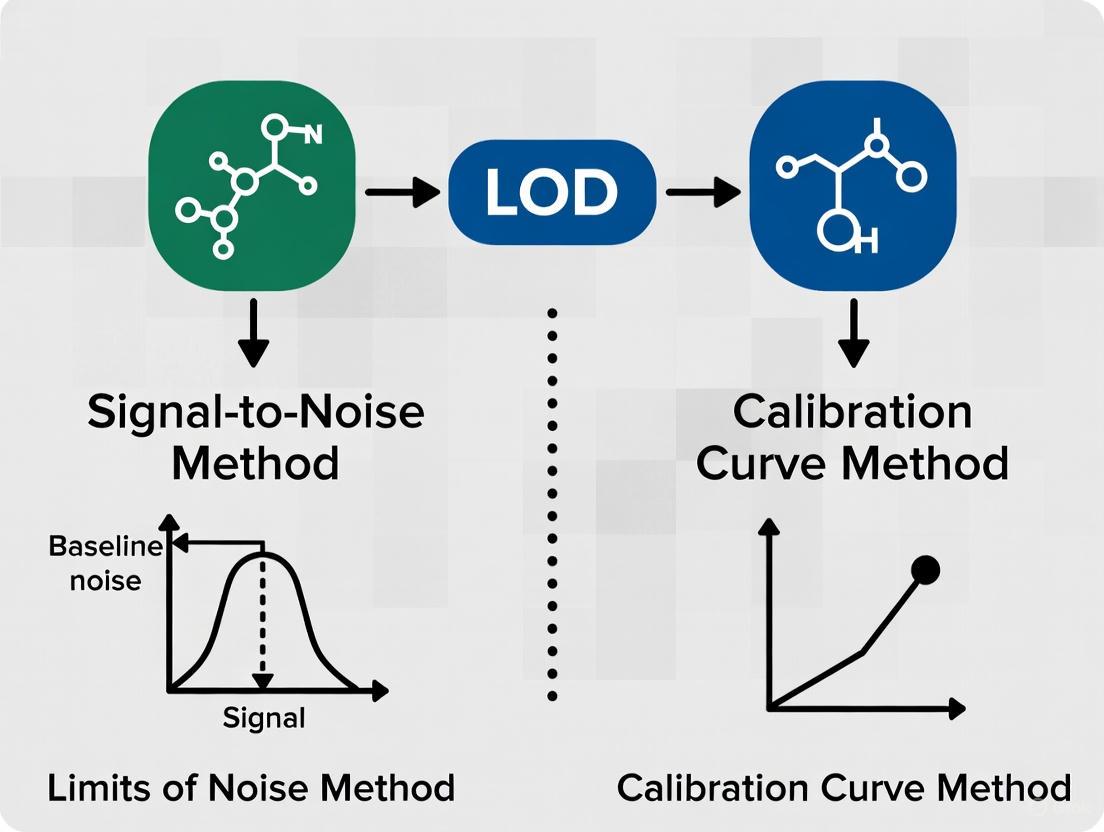
Method Comparison and Workflow Integration

The following diagram illustrates the conceptual relationship and decision workflow between LC, LOD, and LOQ in analytical method validation:

Comparative Assessment of Determination Methods

Research comparing these determination approaches reveals significant methodological differences. A 2024 study published in Scientific Reports found that the classical statistical strategy based on calibration curve parameters provided underestimated values of LOD and LOQ compared to graphical validation approaches like uncertainty profiles [8]. The uncertainty profile method, based on tolerance intervals and measurement uncertainty, provided more realistic assessments and precise uncertainty estimates [8].

The signal-to-noise and calibration curve methods may yield different results for the same analytical method [7] [8]. The S/N approach is more susceptible to operator interpretation, particularly with manual baseline measurements, while the calibration curve method depends heavily on proper experimental design in the low concentration range [7] [6]. From a regulatory perspective, justification for the chosen method is not required, but scientific justification remains important for method robustness [7].

Essential Research Reagents and Materials

The table below outlines key reagents and materials essential for conducting LOD, LOQ, and LC determinations in analytical method validation.

Reagent/Material	Function in Analysis	Critical Specifications
Primary Reference Standard	Calibration curve preparation; known purity material for accurate concentration assignment	Certified purity, stability, proper storage conditions
Blank Matrix	Determination of LC (limit of blank); assessment of background interference	Commutable with patient specimens, analyte-free confirmation
Low Concentration QC Materials	Empirical determination of LOD and LOQ; verification of calculated limits	Commutability, concentration near expected limits, stability
Internal Standard (where applicable)	Normalization of analytical response; improvement of precision	Isotopically labeled (MS methods) or structurally similar analog
Mobile Phase Components	Chromatographic separation; signal optimization	HPLC/MS grade purity, low UV cutoff (for UV detection), freshly prepared

The determination of LOD, LOQ, and LC represents a critical component of analytical method validation, providing essential information about method capability at low analyte concentrations. The signal-to-noise method offers practical simplicity and direct instrument assessment, while the calibration curve approach provides statistical rigor through regression analysis. Emerging methodologies like uncertainty profiles present promising alternatives that incorporate tolerance intervals and measurement uncertainty for more realistic assessments. For researchers and drug development professionals, method selection should consider regulatory context, analytical requirements, and the need for statistical defensibility. As methodological comparisons demonstrate, these approaches are not always equivalent, underscoring the importance of appropriate experimental design and verification in establishing reliable limits for quantitative analytical methods.

In analytical chemistry, particularly during method validation, the limit of detection (LOD) represents the lowest concentration of an analyte that can be reliably detected by an analytical method [9]. The determination of this critical value is intrinsically linked to statistical error theory, specifically the concepts of false positives (Type I errors) and false negatives (Type II errors) [9] [10]. These errors represent the fundamental trade-off between sensitivity and specificity in analytical measurements, directly impacting the reliability of detection capability claims.

When analyzing samples with concentrations near the detection limit, analysts face a decision: declare an analyte "detected" or "not detected" based on the measured signal. This binary decision creates inherent risk. If we analyze many blank samples (containing no analyte), the results will form a distribution around zero with a certain standard deviation (σ₀) due to experimental error [9]. Setting a critical level (Lc) as a decision threshold establishes a boundary: signals above Lc indicate detection, while those below indicate non-detection [9]. This threshold directly controls the probability of statistical errors, forming the foundation for LOD determination methodologies across scientific disciplines.

Theoretical Foundation: Type I and Type II Errors

Defining False Positives and False Negatives

Type I error (false positive) occurs when a true null hypothesis is incorrectly rejected [10]. In detection limit context, this means concluding an analyte is present when it is actually absent [9] [11]. The probability of committing a Type I error (α) represents the risk of false positives, typically set at 5% (α = 0.05) in analytical applications [9]. Visually, this corresponds to the portion of the blank distribution that exceeds the critical level Lc [9].

Conversely, Type II error (false negative) occurs when a false null hypothesis is not rejected [10]. For detection limits, this means failing to detect an analyte that is actually present [9] [11]. The probability of committing a Type II error is denoted by β [10]. The modern definition of LOD incorporates this probability, defining LOD as the true net concentration that will lead to the conclusion that the analyte is present with probability (1-β) [9]. This statistical framework ensures the LOD accounts for both types of potential misclassification.

The Error Relationship Visualization

The relationship between these errors, critical level, and detection limit can be visualized through their probability distributions:

Statistical Decision Framework for Detection Limits - This diagram illustrates the relationship between blank and analyte distributions, critical level (Lc), LOD, and associated error probabilities that form the statistical basis of detection capability.

The critical level Lc is calculated as Lc = z₁₋α × σ₀, where z₁₋α is the critical value from the standardized normal distribution at the chosen significance level α [9]. When α and β are both set to 0.05, and assuming constant standard deviation between blank and LOD concentrations, the detection limit can be expressed as LD = 3.3 × σ₀ [9]. This statistical foundation explains the origin of the factor 3.3 in the ICH-recommended LOD formula LOD = 3.3 × σ/S, where S is the slope of the calibration curve [4] [2].

LOD Determination Methods: Comparative Analysis

Methodological Approaches and Their Statistical Foundations

The International Conference on Harmonization (ICH) Q2(R1) guideline recognizes three primary approaches for determining LOD: visual evaluation, signal-to-noise ratio, and the calibration curve method [4] [2]. Each method implicitly or explicitly addresses the statistical error trade-offs between false positives and false negatives.

Table 1: Comparison of LOD Determination Methods

Method	Statistical Basis	Type I Error Control	Type II Error Control	Typical Application Context
Signal-to-Noise Ratio [2]	Direct comparison of analyte signal to background noise variability	Fixed by S/N = 3:1 ratio convention	Implicitly controlled through the fixed ratio	Chromatographic methods with measurable baseline noise
Calibration Curve [4]	Based on standard deviation of response and slope of calibration curve	α ≈ 0.05 through 3.3 factor in LOD = 3.3σ/S	β ≈ 0.05 through statistical derivation	Instrumental methods where calibration curve can be obtained near LOD
Visual Evaluation [2]	Empirical determination by analyst observation	Variable, depends on analyst stringency	Variable, depends on analyst sensitivity	Non-instrumental methods (e.g., microbial inhibition)

The signal-to-noise approach is commonly applied in chromatographic methods, where the LOD is defined as the concentration that yields a signal-to-noise ratio of 3:1 [2]. This empirical approach implicitly controls error probabilities by establishing a fixed threshold that significantly exceeds typical background fluctuations, thereby reducing false positives while maintaining reasonable detection capability.

The calibration curve method, mathematically expressed as LOD = 3.3 × σ/S, directly incorporates the statistical error framework into its derivation [4] [7]. The factor 3.3 specifically corresponds to the sum of z-values for α = β = 0.05 (approximately 1.645 + 1.645 = 3.29, rounded to 3.3) when standard deviations at zero concentration and at LOD are assumed equal [9]. This method uses the standard error from regression analysis as an estimate of measurement variability, providing a statistically robust approach that explicitly accounts for both Type I and Type II error probabilities.

Experimental Protocols for LOD Determination

Calibration Curve Method Protocol

For the calibration curve method, ICH Q2(R1) recommends using "a specific calibration curve studied using samples containing an analyte in the range of LOD" [7]. The experimental protocol involves:

• Sample Preparation: Prepare a minimum of 5 standard solutions at concentrations in the range of the suspected LOD, typically with the highest concentration not exceeding 10 times the presumed LOD [7].

• Analysis: Analyze each concentration with a minimum of 3 replicates following the complete analytical procedure [7].

• Regression Analysis: Perform linear regression analysis on the concentration-response data. From the regression output, obtain the slope (S) and the standard deviation (σ), which can be either the residual standard deviation or the standard deviation of the y-intercept [4] [7].

• Calculation: Apply the formula LOD = 3.3 × σ/S, ensuring all parameters are in consistent units [4]. The LOQ is similarly calculated as LOQ = 10 × σ/S [4] [2].

• Validation: The calculated values must be experimentally verified by analyzing a suitable number of samples (typically n=6) prepared at the estimated LOD concentration to demonstrate reliable detection [4].

Signal-to-Noise Method Protocol

For the signal-to-noise method, the experimental approach involves:

• Sample Preparation: Prepare standard solutions with decreasing concentrations in the suspected LOD region [2].

• Chromatographic Analysis: Inject samples and measure the signal response at each concentration [9].

• Noise Measurement: Measure the baseline noise in a blank injection, typically over a region equivalent to 20 times the peak width at half height [9].

• Ratio Determination: Calculate the signal-to-noise ratio (S/N) for each concentration, where S is the analyte signal and N is the background noise [9] [2].

• LOD Determination: Identify the concentration where S/N ≈ 3:1 as the LOD [2].

Comparative Method Performance and Research Context

Statistical Reliability and Error Control

Recent research comparing LOD determination methods reveals significant differences in their statistical performance and practical reliability. A 2025 study published in Scientific Reports compared approaches for assessing detection and quantitation limits in bioanalytical methods and found that "the classical strategy based on statistical concepts provides underestimated values of LOD and LOQ" compared to graphical validation approaches like uncertainty profiles [8].

The calibration curve method generally provides more statistically defensible LOD estimates because it explicitly incorporates variability through the standard deviation term and accounts for the sensitivity of the method through the slope parameter [4] [7]. This approach directly addresses both Type I and Type II error probabilities in its derivation, making it scientifically more rigorous than the signal-to-noise method, which relies on fixed, arbitrary ratios [4].

Table 2: Error Trade-offs in LOD Determination Methods

Methodological Consideration	Impact on False Positives	Impact on False Negatives	Practical Implications
Sample Replication [9]	Reduces both error types through better variance estimation	Reduces both error types through better variance estimation	Increased analysis time and cost
Calibration Range Selection [7]	Critical for accurate σ estimation	Critical for accurate slope estimation	Requires preliminary LOD estimate
Assumption of Variance Homogeneity [7]	Underestimated if variance increases near LOD	Overestimated if variance increases near LOD	Can lead to inaccurate error control
Analyst Stringency in Visual Evaluation [2]	Highly variable between analysts	Highly variable between analysts	Poor reproducibility between laboratories

The fundamental challenge in LOD determination remains the inherent trade-off between Type I and Type II errors. As noted in chromatographic literature, "defining LC in such a way that the risk is limited to, for instance, 5% (α = 0.05) seems a more logical decision in most situations" for false positives, but this necessarily increases the LOD to control false negatives [9]. This statistical reality means that no method can simultaneously minimize both error probabilities—improving one necessarily worsens the other, requiring analysts to strategically balance these risks based on their specific application requirements [9] [11].

Research Reagent Solutions for LOD Studies

Table 3: Essential Research Materials for LOD Determination Studies

Reagent/Material	Function in LOD Studies	Critical Quality Attributes
Certified Reference Standards [7]	Provides known analyte concentrations for calibration curves	Purity, stability, traceability to reference materials
Appropriate Matrix Blanks [12]	Distinguishes analyte signal from matrix background	Represents actual sample matrix without target analyte
Chromatographic Solvents [4]	Mobile phase preparation and sample reconstitution	Low UV cutoff, HPLC grade, minimal impurity profile
Sample Preparation Materials [7]	Extraction, purification, and concentration of analytes	Low analyte background, consistent recovery performance

The determination of detection limits in analytical chemistry remains fundamentally grounded in statistical error theory, specifically the balanced control of false positives (Type I errors) and false negatives (Type II errors). While multiple methodological approaches exist for LOD determination, the calibration curve method provides the most direct connection to statistical principles through its explicit incorporation of both α and β error probabilities in the derivation of the 3.3 factor. The signal-to-noise method, while practically convenient, relies on conventional ratios that only indirectly address underlying statistical error trade-offs.

Contemporary research continues to refine LOD determination methodologies, with emerging approaches like uncertainty profiles offering promising alternatives to classical methods [8]. Regardless of the specific technique employed, analysts must recognize that the statistical framework of hypothesis testing forms the foundation of all detection capability assessments. Effective method validation therefore requires not only technical competence in executing analytical procedures but also a thorough understanding of the statistical principles governing error probabilities in detection decisions, enabling informed trade-offs between false positive and false negative risks based on the specific requirements of each analytical application.

The Limit of Detection (LOD) represents a fundamental figure of merit in analytical chemistry, defined as the lowest quantity or concentration of a component that can be reliably detected with a given analytical method. Its determination remains one of the most controversial subjects in analytical chemistry, with multiple definitions and calculation methods contributing to ongoing scientific debate. International organizations including IUPAC, ICH, EPA, and ACS have attempted to establish consensus definitions and estimation guidelines, yet the topic continues to evolve with new methodologies and applications. Understanding the similarities and differences between these guidelines is essential for researchers, scientists, and drug development professionals who must select appropriate LOD determination methods based on their specific analytical requirements, regulatory constraints, and methodological considerations.

The fundamental concept of detection relies on the ability to discriminate between a true analyte signal and background noise or blank measurements. This discrimination inherently involves statistical risks: the probability of false positives (Type I error, α) where an analyte is falsely reported as present, and the probability of false negatives (Type II error, β) where an analyte is present but not detected. Modern LOD definitions incorporate both error types, establishing a performance characteristic that informs analysts about the minimum analyte level a method can detect with a specified degree of confidence. This article compares the perspectives of major international guidelines, providing a structured framework for selecting and implementing LOD determination methods in pharmaceutical and environmental analysis.

Comparative Analysis of International Guidelines

The following sections provide a detailed examination of how different international organizations approach LOD determination, highlighting their statistical foundations, methodological requirements, and appropriate applications.

International Union of Pure and Applied Chemistry (IUPAC)

Statistical Foundation and Definitions IUPAC provides one of the most statistically rigorous frameworks for LOD determination. The organization defines LOD as "the smallest concentration or absolute amount of analyte that has a signal significantly larger than the signal from a suitable blank." This definition emphasizes the need for statistical significance in distinguishing analyte signals from blank measurements. According to IUPAC, the critical level (LC) represents the value at which the decision is made whether the analyte is detected, calculated as LC = z₁₋α × σ₀, where z₁₋α is the critical value from the standardized normal distribution for the chosen significance level α (typically 5%), and σ₀ is the standard deviation of the blank measurements [9].

The IUPAC approach further defines the detection limit (LD) as the true net concentration that will lead to the conclusion that the analyte concentration is greater than that of the blank with probability (1-β). The formula expands to LD = LC + (z₁₋β × σD), where z₁₋β relates to the acceptable false negative rate β, and σD is the standard deviation at the detection limit. When α and β are both set at 0.05 and assuming constant variance, this simplifies to LD = 3.3 × σ₀ [9] [13]. For situations where standard deviation must be estimated from a limited number of replicates, IUPAC recommends replacing z-values with t-values from the Student's t-distribution, resulting in LD = (t₁₋α + t₁₋β) × s₀ when α = β [9].

Practical Implementation The recommended procedure for estimating LOD according to IUPAC guidelines involves analyzing a minimum of 10 portions of a test sample with concentration near the expected detection limit following the complete analytical procedure. The responses are converted to concentrations, and the standard deviation is calculated. The LOD is then computed using the appropriate statistical formula based on the number of replicates and desired confidence levels [9].

International Council for Harmonisation (ICH)

Framework for Pharmaceutical Analysis The ICH Q2(R1) guideline provides validation parameters for analytical procedures in pharmaceutical development and manufacturing. For LOD determination, ICH recognizes two primary approaches: visual evaluation and signal-to-noise ratio. The visual method involves analyzing samples with known concentrations of analyte and establishing the minimum level at which detection is feasible. The signal-to-noise approach compares measured signals from samples with known low concentrations of analyte with those of blank samples, establishing the minimum concentration at which the analyte can be reliably detected [14].

Signal-to-Noise Requirements ICH typically accepts a signal-to-noise ratio of 3:1 for declaring detection capability. This approach is particularly applicable to chromatographic methods and other techniques that display baseline noise. The guideline acknowledges that LOD can also be determined based on the standard deviation of the response or the slope of the calibration curve, using the formula LOD = 3.3σ/S, where σ is the standard deviation of the response and S is the slope of the calibration curve [14]. The ICH approach is specifically designed for pharmaceutical applications and aligns with requirements for method validation in drug development and quality control.

United States Environmental Protection Agency (EPA)

Method Detection Limit (MDL) Procedure The EPA approach focuses on the Method Detection Limit (MDL), defined as "the minimum measured concentration of a substance that can be reported with 99% confidence that the measured concentration is distinguishable from method blank results." The current procedure (Revision 2, 2016) represents a significant evolution from previous versions, incorporating both spiked samples (MDLS) and method blanks (MDLb) in the calculation [15].

Implementation Requirements The EPA procedure requires analysis of at least seven spiked samples and seven method blanks, ideally analyzed throughout the year to represent laboratory performance under varying conditions rather than a single optimal performance period. The MDL is calculated as the higher of the two values (MDLS or MDLb), reflecting the EPA's recognition that background contamination can be as significant as instrumental sensitivity in determining practical detection limits. For the spiked samples, the MDL is derived from the product of the standard deviation of the replicate measurements and the appropriate Student's t-value for the 99% confidence level with n-1 degrees of freedom [15]. This approach emphasizes real-world performance over ideal conditions, capturing instrument drift and variations in equipment conditions throughout the year.

American Chemical Society (ACS)

Environmental Applications Focus The ACS Committee on Environmental Improvement provides specific guidance for environmental analysis. The approach defines LOD as the value at which the sample value is significantly different from the value at the zero-concentration sample at a given confidence level of 95%. The ACS formula is expressed as LOD = 4.6σ, where σ represents the standard deviation of blank replicates measured more than 20 times [13].

Statistical Basis The ACS approach employs a higher multiplier (4.6 versus IUPAC's 3.3) to achieve the 95% confidence level for detection, reflecting the stringent requirements for environmental monitoring where false positives and negatives can have significant regulatory implications. This method requires extensive replication to establish reliable estimates of blank variability, making it more resource-intensive but statistically robust for its intended applications [13].

Table 1: Comparison of LOD Definitions and Statistical Foundations

Organization	Definition	Statistical Formula	Confidence Level	Primary Application
IUPAC	Smallest concentration with signal significantly larger than blank	LOD = 3.3 × σ₀ (for α=β=0.05)	~95% for α=β=0.05	Fundamental analytical chemistry
ICH	Lowest amount detectable with acceptable S/N	Visual or S/N = 3:1 or LOD = 3.3σ/S	Not specified	Pharmaceutical analysis
EPA	Minimum concentration distinguishable from method blank with 99% confidence	MDL = t₉₉ × s (n=7-16 replicates)	99%	Environmental monitoring
ACS	Value significantly different from zero-concentration sample	LOD = 4.6 × σ	95%	Environmental analysis

Methodological Approaches: Signal-to-Noise vs. Calibration Curve

The determination of LOD primarily follows two methodological pathways: the signal-to-noise approach and the calibration curve method. Each approach has distinct advantages, limitations, and appropriate applications within analytical chemistry.

Signal-to-Noise Ratio Approach

Fundamental Principles The signal-to-noise (S/N) approach represents one of the most widely practiced methods for LOD determination, particularly in chromatographic analysis. This method calculates LOD as the concentration providing a signal-to-noise ratio of three. The procedure involves measuring standard solutions with decreasing concentrations until a peak is found whose height is three times taller than the maximum height of the baseline noise measured adjacent to the chromatographic peak [9]. The International Council for Harmonisation, United States Pharmacopeia (USP), and European Pharmacopoeia (EP) all describe variations of this approach, though with differing implementation details [9] [16].

Regulatory Variations and Requirements The European Pharmacopoeia defines signal-to-noise ratio as S/N = 2H/h, where H is the height of the peak corresponding to the component in the chromatogram obtained with the prescribed reference solution, measured from the maximum of the peak to the extrapolated baseline of the signal observed over a distance equal to 20 times the width at half-height. The parameter h represents the range of the background noise in a chromatogram obtained after injection of a blank, observed over the same interval around the time where the peak would be found [9]. In contrast, the USP defines S/N = 2h/hₙ, where h is the height of the peak and hₙ is the difference between the largest and smallest noise values over a distance at least five times the peak width at half-height [16].

Limitations and Considerations While widely used, the S/N approach faces several significant limitations. First, it completely ignores sampling and sample preparation as sources of variability, estimating LOD only for the instrumental step. When determined from a single chromatogram, it fails to account for variability in the injection process [17]. Additionally, in certain instruments like ion-traps used in MRM mode, noise can approach zero, resulting in infinite S/N ratios regardless of peak size or shape [17]. The method also depends heavily on how and where noise is measured, with different guidelines specifying varying time windows for noise assessment [17] [16].

Calibration Curve Method

Statistical Foundation The calibration curve method, endorsed by IUPAC and other statistical approaches, determines LOD based on the standard deviation of the response and the slope of the calibration curve. The fundamental formula is LOD = 3.3 × σ/S, where σ is the standard deviation of the response (residual standard deviation of the regression line or standard deviation of y-intercepts) and S is the slope of the calibration curve [18] [14]. This approach accounts for both the sensitivity of the method (through the slope) and the variability (through the standard deviation), providing a more comprehensive statistical foundation.

Implementation Protocols To implement this approach, analysts prepare a calibration curve with a minimum of five concentrations, ideally in triplicate, spanning the expected range from blank to levels slightly above the anticipated LOD. The standard deviation can be determined through multiple approaches: from the standard deviation of blank measurements, from the residual standard deviation of the calibration curve regression, or from the standard deviation of y-intercepts of regression lines [9] [17]. The calibration curve should be constructed using the same sample preparation and analysis procedures as actual samples, ensuring that the estimated LOD reflects all sources of method variability.

Advantages Over S/N Approach The calibration curve method offers several distinct advantages. It incorporates method precision through the standard deviation estimate, accounts for method sensitivity through the calibration slope, and when properly designed, reflects all sources of variability including sample preparation and matrix effects. Furthermore, this approach aligns with the propagation of errors method, which includes terms for experimental uncertainty in both the slope and y-intercept of the calibration curve, addressing limitations of the simple IUPAC method [19]. As noted in chromatographic forums, this approach makes sense because "limits of detection are directly related to probabilities, and limits of quantification are directly related to percentage errors on the measurements" [17].

Table 2: Comparison of LOD Determination Methodologies

Aspect	Signal-to-Noise Approach	Calibration Curve Approach
Fundamental Basis	Ratio of peak height to baseline noise	Statistical parameters from calibration data
Key Parameters	Peak height, baseline noise	Standard deviation of response, calibration slope
Regulatory Acceptance	ICH, USP, EP	IUPAC, EPA, ACS
Sources of Variability	Primarily instrumental noise	Includes sample prep, matrix effects, and instrumental variability
Implementation Complexity	Simple, direct measurement	Requires multiple standard concentrations
Applicability	Chromatography, spectroscopy	All quantitative analytical methods
Limitations	Ignores sample prep variability, injection variability	Requires careful experimental design, more resources

Experimental Protocols and Workflows

Implementing appropriate experimental protocols is essential for accurate LOD determination. The following sections provide detailed methodologies for both primary approaches.

Signal-to-Noise Protocol for Chromatographic Methods

Sample Preparation

• Prepare a blank sample containing all components except the analyte.
• Prepare a reference solution at a concentration expected to yield a signal-to-noise ratio between 3:1 and 10:1.
• Ensure both solutions undergo identical sample preparation procedures.

Instrumental Analysis

• Inject the blank sample and record the chromatogram.
• Measure the baseline noise over a region free from chromatographic peaks. According to EP guidelines, this region should span a distance equal to 20 times the peak width at half-height [9] [16].
• Inject the reference solution and record the chromatogram.
• Measure the height of the analyte peak from the maximum response to the extrapolated baseline.

Calculation

• Calculate signal-to-noise ratio using the appropriate formula (EP: S/N = 2H/h; USP: S/N = 2h/hₙ).
• If the ratio is approximately 3, the concentration is the LOD.
• If the ratio differs significantly from 3, prepare additional reference solutions at adjusted concentrations and repeat until the 3:1 ratio is achieved.

Calibration Curve Protocol for LOD Determination

Experimental Design

• Prepare a minimum of five standard solutions spanning concentrations from blank to slightly above the expected LOD.
• Include a minimum of three replicates at each concentration level.
• Process all standards through the complete analytical procedure, including any sample preparation steps.

Data Collection and Analysis

• Analyze all standards in random order to avoid systematic bias.
• Record the instrument response for each standard and replicate.
• Construct a calibration curve with concentration on the x-axis and response on the y-axis.
• Perform linear regression analysis to determine the slope (S) and the standard deviation of the residuals (sᵧ/ₓ) or the standard deviation of blank measurements.

LOD Calculation

• Calculate LOD using the formula: LOD = 3.3 × sᵧ/ₓ / S
• For increased robustness, particularly with limited replicates, use the formula: LOD = (t₁₋α + t₁₋β) × s₀ / S, where t-values correspond to the appropriate degrees of freedom and confidence levels.

The following workflow diagram illustrates the decision process for selecting and implementing the appropriate LOD determination method:

Diagram Title: LOD Determination Method Selection Workflow

Essential Research Reagent Solutions and Materials

Implementing robust LOD determination requires specific materials and reagents tailored to the analytical method and sample matrix. The following table details essential research solutions for LOD studies.

Table 3: Essential Research Reagent Solutions for LOD Determination

Reagent/Material	Function	Specification Requirements	Application Notes
High-Purity Analytical Standards	Calibration reference	Certified reference materials with documented purity ≥95%	Prepare fresh stock solutions; verify stability
Matrix-Matched Blank Samples	Blank measurement	Representative matrix without target analytes	Should contain all matrix components except analyte
High-Purity Solvents	Standard preparation and extraction	HPLC or GC grade with low background interference	Test for interference in target analyte regions
Internal Standards	Correction for variability	Stable isotopically labeled analogs of target analytes	Use for mass spectrometry methods
Derivatization Reagents	Analyte detection enhancement	High purity with minimal side reactions	Optimize for specific analyte detection
Solid Phase Extraction Cartridges	Sample cleanup and concentration	Appropriate sorbent for target analytes	Minimize background interference
Mobile Phase Additives	Chromatographic separation	MS-grade for mass spectrometry	Reduce chemical noise in detection

The comparison of international guidelines reveals both convergence and divergence in LOD determination methodologies. While all guidelines seek to establish the lowest reliably detectable analyte concentration, their statistical approaches, implementation requirements, and application domains differ significantly. The selection between signal-to-noise and calibration curve approaches should be guided by regulatory requirements, methodological considerations, and practical constraints.

For pharmaceutical applications under ICH guidelines, the signal-to-noise approach offers simplicity and direct applicability to chromatographic methods commonly used in drug analysis. For environmental monitoring following EPA protocols, the Method Detection Limit procedure provides comprehensive assessment incorporating real-world variability. For fundamental research and method development, the IUPAC calibration curve approach offers statistical rigor and comprehensive variability assessment.

The ongoing development of tools like the Red Analytical Performance Index (RAPI), which consolidates multiple performance criteria including LOD into a unified scoring system, represents the future of analytical method assessment [20]. Regardless of the selected approach, transparent reporting of methodology, complete documentation of experimental parameters, and appropriate validation are essential for credible LOD determination in research and regulatory contexts.

In pharmaceutical analysis and drug development, accurately determining the lowest concentrations of an analyte is paramount. Two critical performance parameters form the foundation of this capability: the Limit of Detection (LOD) and the Limit of Quantification (LOQ). The LOD is defined as the lowest concentration of an analyte that can be reliably detected—but not necessarily quantified—under stated experimental conditions, answering the question "Is it there?" [21] [2]. In contrast, the LOQ represents the lowest concentration that can be quantitatively determined with acceptable precision and accuracy, answering the question "How much is there?" [8] [2]. This distinction is not merely semantic; it represents a fundamental difference in the confidence level of the analytical result, with the LOQ requiring a significantly higher degree of certainty for reliable measurement.

The international guideline ICH Q2(R1) recognizes multiple approaches for determining these limits, primarily the signal-to-noise ratio (S/N) and the calibration curve method [5] [2] [7]. While both are academically and regulatorily accepted, they operate on different principles and can yield significantly different results, leading to potential confusion or misinterpretation in analytical data. This guide provides an objective comparison of these methodologies, supported by experimental data, to inform researchers and scientists in selecting the most appropriate approach for their specific analytical challenges.

Methodological Foundations: S/N Ratio vs. Calibration Curve

The Signal-to-Noise (S/N) Ratio Approach

The S/N method is one of the most visually intuitive techniques for determining LOD and LOQ, particularly for chromatographic methods that exhibit baseline noise [5] [2]. This approach involves comparing the measured signal from a sample containing a low concentration of analyte with those of blank samples to establish the minimum concentration at which the analyte can be reliably detected or quantified.

• Fundamental Principle: The method is based on the direct comparison of the analyte signal height (or amplitude) to the peak-to-peak noise of the baseline in a blank sample [9] [5].
• Standard Acceptance Criteria: According to ICH Q2(R1), a signal-to-noise ratio between 2:1 and 3:1 is generally considered acceptable for estimating the detection limit, while a ratio of 10:1 is typical for the quantitation limit [5] [2]. It is important to note that the upcoming ICH Q2(R2) revision is expected to mandate a S/N of 3:1 for LOD, eliminating the 2:1 option [5].
• Practical Implementation: In practice, the baseline noise is measured from a peak-free section of the chromatogram, either from the current run or a previous blank run. The LOD is then defined as the concentration that yields a peak height three times the noise level, while the LOQ yields a peak height ten times the noise level [5].

The Calibration Curve Approach

The calibration curve method offers a more statistically rigorous approach to determining LOD and LOQ, relying on the standard deviation of the response and the slope of the calibration curve [21] [7].

• Fundamental Principle: This method utilizes the variability in response at low analyte concentrations to estimate the limits of detection and quantification. The standard deviation (σ) can be derived from different statistical parameters, most commonly the residual standard deviation of the regression line or the standard deviation of the y-intercepts of regression lines [2] [7].
• Calculation Methodology: The LOD and LOQ are calculated using the formulas:
  • LOD = 3.3 × σ / S [2] [7]
  • LOQ = 10 × σ / S [2] Where σ is the standard deviation of the response and S is the slope of the calibration curve.
• Experimental Considerations: A specific calibration curve should be studied using samples containing the analyte in the range of the LOD, not the entire working range of the method. This is crucial because using a "normal" calibration line with higher values would shift the center to a higher value, resulting in an overestimated detection limit [7].

Experimental Workflow Comparison

The fundamental differences in how the S/N ratio and calibration curve methods approach LOD/LOQ determination can be visualized in their experimental workflows.

Comparative Experimental Data Across Analytical Fields

Pharmaceutical Analysis: Carbamazepine and Phenytoin

A 2024 study compared different approaches for calculating LOD and LOQ in an HPLC-UV method for analyzing the drugs carbamazepine and phenytoin, revealing significant variability in results depending on the method used [22].

Table 1: Comparison of LOD and LOQ Values for Pharmaceutical Compounds Using Different Calculation Methods

Analytical Method	Compound	S/N Method LOD	Calibration Curve LOD	S/N Method LOQ	Calibration Curve LOQ
HPLC-UV	Carbamazepine	Lowest value	Highest value	Lowest value	Highest value
HPLC-UV	Phenytoin	Lowest value	Highest value	Lowest value	Highest value

The study concluded that the signal-to-noise ratio method provided the lowest LOD and LOQ values for both drugs, while the standard deviation of the response and slope method resulted in the highest values [22]. This highlights the substantial variability in sensitivity parameters depending on the calculation method chosen.

Food Safety: Aflatoxin in Hazelnuts

A 2015 study examining aflatoxin analysis in hazelnuts using AOAC Method 991.31 compared visual evaluation, signal-to-noise, and calibration curve approaches for determining LOD and LOQ [21].

Table 2: Method Comparison for Aflatoxin Analysis in Hazelnuts

Calculation Method	Key Findings	Advantages	Limitations
Visual Evaluation	Provided much more realistic LOD and LOQ values	Based on actual detection capability	Subjective element in peak identification
Signal-to-Noise	Standard approach with defined ratios	Simple, instrument-friendly	Does not account for sample prep variability
Calibration Curve	Calculated using residual standard deviation	Statistical robustness	Requires multiple calibration curves

The study concluded that the visual evaluation method provided much more realistic LOD and LOQ values compared to the other approaches [21].

Bioanalytical Methods: Sotalol in Plasma

A 2025 study in Scientific Reports compared classical statistical approaches with graphical tools (uncertainty profile and accuracy profile) for assessing LOD and LOQ in an HPLC method for determining sotalol in plasma [8]. The research found that the classical strategy based on statistical concepts provided underestimated values of LOD and LOQ, while the graphical tools offered a more relevant and realistic assessment [8]. The values found by uncertainty and accuracy profiles were in the same order of magnitude, with the uncertainty profile method providing a precise estimate of the measurement uncertainty [8].

Statistical and Regulatory Considerations

Understanding False Positives and Negatives

The statistical foundation of LOD and LOQ determination involves managing the risks of false positives (Type I error, α) and false negatives (Type II error, β) [9]. When analyzing blank samples, the results distribute around zero with a given standard deviation (σ₀). Establishing a critical level (LC) allows analysts to decide whether an analyte is present, but this decision always carries a statistical risk [9].

• False Positive Risk: Setting LC too low increases the probability (α) of concluding an analyte is present when it is not [9].
• False Negative Risk: Setting LOD at the critical level would result in approximately 50% of low-concentration samples being incorrectly reported as not detected [9].
• Modern LOD Definition: The International Organization for Standardization (ISO) defines LOD as the true net concentration that will lead, with probability (1-β), to the conclusion that the concentration of the component in the material analyzed is greater than that of a blank sample [9].

Regulatory Perspectives and Guidelines

Various international regulatory bodies provide guidelines for LOD and LOQ determination, with some variations in acceptable approaches.

• ICH Q2(R1): Recognizes visual evaluation, signal-to-noise ratio, and standard deviation of the response (calibration curve) as acceptable methods [5] [2].
• Upcoming ICH Q2(R2): Expected to implement stricter criteria, specifically requiring a S/N of 3:1 for LOD estimation rather than the current 2:1-3:1 range [5].
• CLSI EP17 Guideline: Provides a standardized approach for determining LoB (Limit of Blank), LoD, and LoQ in clinical laboratory settings, using specific formulas:
  • LoB = meanblank + 1.645(SDblank) [3]
  • LoD = LoB + 1.645(SD_low concentration sample) [3]

Essential Research Reagent Solutions for LOD/LOQ Studies

Table 3: Key Reagents and Materials for LOD/LOQ Determination Experiments

Reagent/Material	Function in Analysis	Application Examples
Immunoaffinity Columns (IAC)	Cleanup and isolation of extracted analytes	AflaTest-P columns for aflatoxin analysis [21]
HPLC-Grade Solvents	Mobile phase preparation	Methanol, acetonitrile for HPLC analysis [21]
Certified Reference Materials	Calibration and quality control	Aflatoxin standards for hazelnut analysis [21]
Chromatography Columns	Analytical separation	ODS-2 RP-HPLC columns [21]
Internal Standards	Correction for analytical variability	Atenolol for sotalol determination in plasma [8]

The comparative analysis of signal-to-noise versus calibration curve methods for LOD and LOQ determination reveals a complex landscape with no universal "best" approach. Each method has distinct advantages and limitations that make it more or less suitable for specific applications.

For routine quality control in regulated environments where simplicity and compliance are paramount, the signal-to-noise method offers straightforward implementation and alignment with ICH guidelines [5] [2]. However, analysts should be aware of its limitations, particularly its failure to account for sample preparation variability and its potential for over-optimistic results [17].

For method development and research applications where statistical robustness and a comprehensive understanding of method capabilities are required, the calibration curve approach provides a more rigorous foundation [21] [7]. While more labor-intensive, it accounts for variability across the entire analytical process and generates more realistic performance estimates.

The most defensible approach, particularly for method validation, may involve using multiple determination techniques to establish a consensus value. As demonstrated across numerous studies, the methodological choice significantly impacts the reported sensitivity parameters, potentially influencing decisions in drug development, regulatory submissions, and scientific conclusions. Researchers should clearly document their selected methodology and justify its appropriateness for their specific analytical challenge.

A Practical Guide to Implementing S/N and Calibration Curve Methods

In analytical chemistry, the Limit of Detection (LOD) represents the lowest concentration of an analyte that can be reliably distinguished from the absence of that analyte. Among the various approaches for determining LOD, the Signal-to-Noise (S/N) method remains one of the most widely used techniques, particularly in chromatographic and spectroscopic analyses. This method offers a practical balance between empirical assessment and mathematical calculation, providing analysts with a relatively straightforward means of establishing method detection capabilities. The S/N approach is formally recognized in major validation guidelines, including the International Conference on Harmonisation (ICH) Q2(R1) and its upcoming revision, which specifies that "a signal-to-noise ratio between 3:1 or 2:1 is generally considered acceptable for estimating the detection limit" [21] [23].

The fundamental principle underlying the S/N method is that an analyte signal must be sufficiently distinguishable from the ever-present background noise of the analytical system. As ICH Q2(R2) now states more definitively, "A signal-to-noise ratio of 3:1 is generally considered acceptable for estimating the detection limit" [5]. This ratio provides a statistical basis for detection, ensuring that the probability of false positives (Type I errors) remains acceptably low. For quantitative purposes, the Limit of Quantification (LOQ) is typically set at a higher S/N ratio of 10:1, providing sufficient signal confidence for reliable quantification with acceptable precision and accuracy [21] [23] [5].

This guide provides a comprehensive comparison of the S/N method against alternative approaches, particularly the calibration curve method, with supporting experimental data from published studies. By examining the protocols, calculations, and practical implementations of these techniques, analysts can make informed decisions about the most appropriate methodology for their specific analytical challenges.

Theoretical Foundation of the S/N Method

Fundamental Principles and Definitions

The Signal-to-Noise method operates on a straightforward premise: for an analyte to be reliably detected, its signal must be statistically distinguishable from the background noise of the measurement system. The signal refers to the analytical response attributable to the analyte, typically measured as peak height in chromatographic systems or absorption intensity in spectroscopic techniques. The noise represents the random fluctuations in the analytical signal when no analyte is present, arising from various sources including electronic instability, detector limitations, and environmental interference [5].

The mathematical foundation of the S/N method is deceptively simple, with the ratio calculated as:

S/N = Signal Height / Noise Amplitude

Despite this apparent simplicity, practical implementation requires careful consideration of noise measurement methodologies. Two primary approaches exist for quantifying noise:

• Peak-to-peak noise: The difference between the maximum and minimum baseline values over a specified region
• Root mean square (RMS) noise: A statistical measure of the magnitude of varying quantity, providing a more robust estimate of noise power [23]

The relationship between S/N ratios and detection capabilities follows statistical principles. A S/N ratio of 3:1 corresponds to a confidence level of approximately 99.7% that a measured signal represents a true analyte detection rather than random noise fluctuation, assuming a normal distribution of noise [5]. This statistical foundation makes the S/N method both practically accessible and scientifically defensible for establishing detection limits.

Regulatory Acceptance and Guidelines

The S/N method enjoys broad acceptance across regulatory frameworks, though specific implementation details may vary. The ICH Q2(R1) guideline recognizes S/N as one of three acceptable methods for determining LOD and LOQ, alongside visual evaluation and standard deviation-based approaches [23]. The upcoming ICH Q2(R2) revision further clarifies that a S/N ratio of 3:1 is specifically required for LOD estimation, eliminating the previous acceptance of 2:1 ratios [5].

Other regulatory bodies, including the United States Pharmacopeia (USP) and European Pharmacopoeia (EP), also acknowledge the S/N approach, though analysts should note potential differences in calculation methodologies between these organizations [23]. This regulatory acceptance makes the S/N method particularly valuable in pharmaceutical analysis and other highly regulated fields where method validation requirements are stringent.

Step-by-Step Experimental Protocol

Sample Preparation and Instrumentation

The S/N method requires careful preparation of samples designed to produce signals near the expected detection limit. The following protocol outlines a standardized approach:

• Prepare a blank sample containing all matrix components except the analyte of interest. This sample should be representative of the actual test samples to ensure matrix effects are properly accounted for [5].

• Prepare a low-concentration standard at a concentration expected to yield a signal approximately 3-5 times the baseline noise. This may require preliminary experiments to establish the appropriate concentration range [21] [5].

• Analyze the blank sample using the complete analytical method, recording the chromatogram or spectrum in the region where the analyte signal is expected. The analysis should be performed under identical conditions to those used for actual samples [5].

• Analyze the low-concentration standard using the same instrumental conditions, ensuring sufficient replication to account for normal method variability (typically n ≥ 6) [21].

• Maintain consistent instrumental parameters throughout the analysis, as detector settings (e.g., time constant in UV detectors, slit width) can significantly impact both signal and noise measurements [5].

Measurement and Calculation Procedures

Once samples have been analyzed, the S/N ratio calculation proceeds as follows:

• Measure the signal height from the low-concentration standard chromatogram or spectrum. The measurement should be from the baseline to the maximum point of the analyte peak [23] [5].

• Measure the noise amplitude from the blank chromatogram or spectrum. Select a representative region free from interferences, typically immediately adjacent to the analyte retention time. The noise should be measured over a sufficient time window (typically 10-20 times the peak width at baseline) to ensure statistical significance [23].

• Calculate the S/N ratio by dividing the signal height by the noise amplitude:

  • S/N = H / N
  • Where H = signal height and N = noise amplitude [23] [5]

• Verify the LOD and LOQ:

  • If S/N ≈ 3, the concentration corresponds to the LOD
  • If S/N ≈ 10, the concentration corresponds to the LOQ
  • If the measured S/N does not match these targets, adjust the concentration accordingly and repeat the measurements [21] [5]

• Confirm by independent injection of samples at the calculated LOD and LOQ concentrations to ensure consistency between calculated and observed S/N ratios [24].

Figure 1: Step-by-Step Workflow for S/N Method Implementation. This diagram illustrates the complete experimental protocol for determining LOD and LOQ using the signal-to-noise approach, from sample preparation to final verification.

Comparative Experimental Data: S/N vs. Alternative Methods

Direct Method Comparison Studies

Multiple studies have directly compared the S/N method with alternative approaches for LOD determination, revealing significant differences in results and practical implementation. The following table summarizes key findings from these comparative investigations:

Table 1: Experimental Comparison of LOD Determination Methods Across Different Studies

Study Context	S/N Method LOD	Calibration Curve LOD	Visual Evaluation LOD	Key Findings	Reference
Aflatoxin in Hazelnuts (HPLC)	Not specified	Varied based on SD type	1 μg/kg total aflatoxin	Visual method provided more realistic values; calibration curve results depended on using residual SD or y-intercept SD	[21]
Monoclonal Antibody Purity (cIEF)	0.09% (relative concentration)	0.07% (relative concentration)	Not reported	Different techniques produced substantially different results; S/N and calibration curve showed reasonable agreement	[25]
General HPLC Applications	3:1 S/N ratio	Based on SD of response and slope	Subjective assessment	S/N and visual methods can be arbitrary; calibration curve provides more statistical rigor	[23]
Sotalol in Plasma (HPLC)	Not specified	Classical strategy provided underestimated values	Uncertainty profile provided precise estimate	Graphical strategies (uncertainty profile) more reliable than classical statistical approaches	[8]

The data reveals that method selection significantly impacts the determined LOD values, with differences often exceeding an order of magnitude in some applications. This variability underscores the importance of both method selection and transparent reporting of the specific methodology used.

Advantages and Limitations of Each Method

Each LOD determination method presents distinct advantages and limitations that analysts must consider when selecting an appropriate approach:

Table 2: Comparative Analysis of LOD Determination Methodologies

Method	Advantages	Limitations	Ideal Application Context
Signal-to-Noise (S/N)	- Simple, quick implementation- Direct instrumental measurement- Broad regulatory acceptance- Intuitively understandable	- Sensitive to measurement conditions- Noise measurement subjectivity- Dependent on data processing parameters- Limited statistical foundation	- Routine chromatographic analysis- Methods with stable baselines- Screening methods where speed is prioritized
Calibration Curve	- Strong statistical foundation- Accounts for method precision- Less operator-dependent- Utilizes existing validation data	- Requires multiple concentration levels- Assumes linearity near LOD- Sensitive to outlier points- More computationally intensive	- Regulated pharmaceutical methods- Methods requiring robust statistical support- Research applications
Visual Evaluation	- Practical, intuitive approach- Direct assessment of chromatograms- No complex calculations	- Highly subjective- Poor reproducibility between analysts- Difficult to validate and document- Limited regulatory acceptance	- Preliminary method development- Quick assessments during optimization- Supporting data for other methods

The comparative analysis indicates that while the S/N method offers practical advantages for routine applications, methods based on calibration curves may provide greater statistical rigor for regulated environments where demonstration of robust validation is required.

Critical Implementation Considerations

Impact of Data Processing Parameters

The determined S/N ratio is highly dependent on data processing techniques and instrumental parameters, creating significant potential for variability between laboratories and analysts. Several factors critically influence S/N calculations:

• Time constant/filter settings: Electronic filters can reduce apparent noise but may also distort or suppress legitimate analyte signals, particularly near detection limits. Over-use of smoothing filters can artificially improve S/N ratios while actually reducing detection capability [5].

• Noise measurement methodology: The distinction between peak-to-peak noise and RMS noise measurements can yield significantly different S/N values from the same data set. One study noted that "the traditional signal-divided-by noise method gives a value that is half of the one used by the USP and EP" [23].

• Integration parameters: Automated integration algorithms may fail to properly identify peaks near the detection limit, requiring manual intervention that introduces subjectivity [23] [5].

• Baseline selection: The region selected for noise measurement significantly impacts calculated ratios. Noise should be measured "in the current chromatogram or from a previous blank run" in a "peak-free section" [5].

These dependencies highlight the importance of standardizing and thoroughly documenting data processing parameters when using the S/N method for formal method validation.

Regulatory and Practical Recommendations

Based on comparative studies and regulatory guidelines, the following recommendations emerge for implementing S/N methods in regulated environments:

• Use S/N as a confirmatory approach: Given its limitations, the S/N method "should be used primarily for confirmation of less arbitrary calculations" rather than as the sole basis for LOD determination [23].

• Apply realistic S/N thresholds: While ICH specifies a 3:1 ratio for LOD, "in reality with real-life samples and analytical conditions" more conservative values of "SNR between 3:1 and 10:1 for LOD" and "SNR from 10:1 to 20:1 for LOQ" are often appropriate [5].

• Standardize noise measurement protocols: Implement consistent approaches for noise measurement, including defined regions for assessment and standardized data processing parameters, to improve inter-laboratory reproducibility.

• Corroborate with alternative methods: "A quick look at two publications shows that the results differ depending on which method is used to determine the LOD and LOQ" [7]. Using multiple determination approaches provides more robust validation.

• Document all parameters thoroughly: Given the potential for variability, complete documentation of instrumental settings, data processing parameters, and calculation methodologies is essential for method validation.

The Scientist's Toolkit: Essential Research Reagents and Materials

Successful implementation of LOD determination methods requires appropriate laboratory materials and reagents. The following table outlines essential components for conducting S/N-based detection limit studies:

Table 3: Essential Research Materials for LOD Determination Studies

Category	Specific Items	Function/Purpose	Critical Considerations
Reference Standards	- Certified analyte standard- Isotopically labeled internal standards	- Preparation of calibration solutions- Method accuracy verification	- Purity certification- Stability data- Appropriate storage conditions
Matrix Materials	- Blank matrix samples- Artificial matrix formulations	- Assessment of matrix effects- Preparation of fortified samples	- Commutability with real samples- Stability and homogeneity- Representative composition
Chromatographic Supplies	- HPLC/UHPLC columns- Mobile phase components- Sample filtration units	- Separation and detection of analytes- Sample preparation and cleanup	- Column selectivity and efficiency- Chemical purity- Compatibility with detection system
Instrumentation	- High-sensitivity detectors (e.g., DAD, FLD, MS)- Precision injection systems- Data acquisition software	- Signal generation and measurement- Data processing and calculation	- Detection specificity- Injection precision- Data processing capabilities

The Signal-to-Noise method represents a practically accessible approach for LOD determination with broad regulatory acceptance, particularly in chromatographic applications. Its intuitive foundation and straightforward implementation make it valuable for routine analytical applications and initial method development. However, comparative studies consistently demonstrate that the S/N method can yield significantly different results than alternative approaches such as calibration curve methods, visual evaluation, or emerging techniques like uncertainty profiles.

The choice between LOD determination methods should be guided by the specific application context, regulatory requirements, and necessary rigor level. For screening methods where speed and simplicity are prioritized, the S/N method provides sufficient reliability. For regulated methods requiring robust statistical support and minimal subjectivity, calibration curve-based approaches offer greater scientific defensibility. In many cases, a combination of methods, using S/N for initial estimation and calibration curves for validation, represents the most comprehensive approach.

Regardless of the selected methodology, transparent reporting of the specific protocol, including detailed documentation of calculation parameters and experimental conditions, remains essential for generating comparable and reliable detection limit data. This practice ensures analytical methods are truly "fit for purpose" and capable of generating defensible data at the limits of detection.

Thesis Context: This guide provides an objective comparison of methods for determining the Limit of Detection (LOD), focusing on the calibration curve method against the signal-to-noise approach, to inform researchers and drug development professionals on their application and performance.

Theoretical Foundations of LOD Determination

In the validation of analytical and bioanalytical methods, the Limit of Detection (LOD) and Limit of Quantification (LOQ) are two crucial parameters that define the lowest concentrations of an analyte that can be reliably detected and quantified, respectively [8] [2]. The accurate determination of these limits is fundamental to ensuring that an analytical procedure is "fit for purpose," particularly in pharmaceutical development and other regulated fields where measuring very low concentrations of impurities or active compounds is required [3]. The International Conference on Harmonisation (ICH) Q2(R1) guideline outlines several accepted approaches for determining these limits, primarily the visual evaluation, the signal-to-noise ratio, and the method based on the standard deviation of the response and the slope of the calibration curve [4] [2].

The calibration curve method, expressed by the formula LOD = 3.3 σ / S, is grounded in robust statistical principles [4]. In this equation, 'σ' represents the standard deviation of the response, and 'S' is the slope of the calibration curve [7] [4]. The factor of 3.3 arises from statistical theory, accounting for a risk of 5% for both false positive and false negative detection events, providing a 95% confidence level for the detection [2]. The underlying assumption is that there is a linear relationship in the region of the suspected LOD, and that the response values are normally distributed and exhibit homogeneous variance across the calibration range [7]. This method shifts the determination of detection limits from potentially subjective assessments to a reproducible, data-driven calculation based on the fundamental performance characteristics of the analytical method itself—its sensitivity (slope) and its variability (standard deviation) at low concentrations.

Experimental Protocols for the Calibration Curve Method

Step-by-Step Procedure

Implementing the calibration curve method for LOD and LOQ determination requires a meticulous experimental setup to ensure accurate and reliable results. The following protocol, synthesizing best practices from multiple sources, provides a detailed roadmap:

• Preparation of Calibration Standards: The cornerstone of this method is the construction of a specific calibration curve using samples with analyte concentrations in the range of the presumed LOD and LOQ [7]. It is critical not to use the standard working calibration curve that spans a much wider range, as its center is shifted to a higher value, which can lead to an overestimation of the LOD [7]. A recommended practice is to prepare the highest concentration for this specific curve at no more than 10 times the presumed detection limit [7]. A minimum of five concentration levels is advisable to establish a reliable regression line.

• Analysis and Data Acquisition: Each calibration standard should be analyzed in replicate, typically three times (n=3), using the complete analytical procedure, including sample preparation [7]. This helps capture the method variability. The instrument response (e.g., peak area in HPLC) for each standard is recorded.

• Linear Regression Analysis: The concentration (x-axis) and the corresponding instrument response (y-axis) data are subjected to linear regression analysis. This can be performed using standard software like Microsoft Excel, which provides a regression output containing the necessary statistical parameters [4]. The key values to extract from this analysis are:

  • The slope (S) of the calibration curve.
  • The standard error of the regression (also known as the residual standard deviation) [4].
  • The standard deviation of the y-intercept can also be used as an estimate for σ [7] [2].

• Calculation of LOD and LOQ: Using the parameters derived from the regression analysis, the LOD and LOQ are calculated as follows:

  • LOD = 3.3 × (Standard Error of Regression) / Slope [4]
  • LOQ = 10 × (Standard Error of Regression) / Slope [4]

• Experimental Verification: The ICH guideline mandates that the calculated LOD and LOQ values are verified through experiment [4]. This involves preparing and analyzing a suitable number of samples (e.g., n=6) at the calculated LOD and LOQ concentrations. The LOD should consistently demonstrate a detectable peak, while the LOQ should demonstrate both acceptable accuracy (e.g., ±15% of the true value) and precision (e.g., ±15% relative standard deviation) [4]. This empirical confirmation is essential for validating the statistically derived limits.

Visualizing the Workflow

The following diagram illustrates the logical sequence and key decision points in the protocol for determining LOD and LOQ via the calibration curve method.

Comparative Performance Analysis

Quantitative Data Comparison

A direct comparison of the different LOD determination methods reveals significant differences in their underlying principles, computational approaches, and the resulting values.

Table 1: Objective Comparison of LOD Determination Methods

Method	Fundamental Principle	Calculation Basis	Typical LOD Result	Key Advantages	Key Limitations
Calibration Curve	Statistical model of response at low concentration	Slope (S) and standard deviation (σ) of regression: LOD=3.3σ/S [4]	Can be more realistic and lower [7]	Robust, statistical foundation; less arbitrary; uses full calibration data [4]	Requires specific low-level curve; results vary with σ estimate (y-intercept vs. residuals) [7] [8]
Signal-to-Noise (S/N)	Instrumental baseline noise	Ratio of analyte signal to background noise: LOD at S/N ≥ 2:1 or 3:1 [21] [2]	Can be arbitrary and higher [21]	Simple, fast, instrument-agnostic [4]	Subjective; ignores sample prep variability; less suitable for non-instrumental methods [4]
Visual Evaluation	Empirical observation	Lowest concentration producing a detectable peak [21] [2]	Considered more realistic in some studies [21]	Intuitive; direct assessment	Highly subjective; dependent on analyst experience; not statistically robust [4]

The performance of these methods is not merely theoretical. A practical example from a study on aflatoxin analysis in hazelnuts using HPLC demonstrated that the visual evaluation method provided much more realistic LOD and LOQ values compared to other approaches [21]. Furthermore, a 2025 study in Scientific Reports comparing methods for sotalol in plasma found that the classical strategy based on statistical concepts (like the calibration curve method) provided underestimated values of LOD and LOQ compared to more modern graphical tools like the uncertainty profile [8]. This indicates that while the calibration curve method is scientifically robust, its results can vary and should be interpreted with an understanding of its potential to underestimate detection limits in certain contexts.

Critical Assumptions and Potential Pitfalls

The calibration curve method, while powerful, relies on several critical assumptions that, if violated, can lead to significant inaccuracies. A primary requirement is that the analytical response must demonstrate linearity in the immediate region of the presumed LOD [7]. If the dose-response relationship deviates from linearity at these low concentrations, the fundamental formula LOD = 3.3σ/S becomes invalid. Furthermore, the method assumes homogeneity of variance (homoscedasticity) across the low-concentration range used to build the curve [7]. If the variance of the instrument response increases or decreases with concentration, the standard deviation (σ) used in the calculation will not be representative.

Another notable pitfall is the variability in results depending on the chosen estimate for the standard deviation (σ). As illustrated in a practical example, calculating the LOD using the standard deviation of the y-intercept versus the residual standard deviation of the regression line can yield different results [7]. For instance, in one experiment, the LOD calculated from the y-intercept SD was 0.61 µg/mL, while the residual SD gave a value of 0.72 µg/mL [7]. This highlights the importance of consistently applying the same approach for σ estimation when comparing methods or performing longitudinal studies. Finally, the calculated LOD and LOQ are only estimates and must be empirically verified by analyzing multiple samples at those concentrations to confirm that they meet the required performance criteria for detection and quantification, a step that is mandated by the ICH guideline [4].

The Scientist's Toolkit: Essential Research Reagents and Materials

The successful implementation of the calibration curve method for LOD determination depends on the use of high-quality materials and reagents. The following table details key items essential for experiments such as aflatoxin analysis in food or drug substance analysis in pharmaceuticals.

Table 2: Essential Research Reagents and Materials for LOD Experiments

Item	Function / Purpose	Example from Literature
Certified Reference Standards	Used to prepare accurate calibration standards and spike samples for recovery studies; ensures traceability and accuracy of results.	Aflatoxin standard solution (R-Biopharm) used for calibration and spiking blank hazelnut samples [21].
Chromatography Columns	Stationary phase for separation; critical for resolving the analyte from matrix interferences, which is essential for accurate detection at low levels.	ODS-2 reversed-phase HPLC column used for aflatoxin separation [21].
Immunoaffinity Columns (IAC)	Sample cleanup and extraction; selectively binds the target analyte to purify it from complex sample matrices, reducing background noise.	AflaTest-P IAC (VICAM) used for cleanup and isolation of aflatoxins from hazelnut samples [21].
HPLC-Grade Solvents	Used as mobile phase components and for sample dissolution; high purity is necessary to minimize baseline noise and ghost peaks.	HPLC gradient grade methanol and acetonitrile used in the mobile phase [21].
Blank Matrix Sample	A real sample known to be free of the analyte; used for preparing calibration standards and spike samples to account for matrix effects.	Toxin-free hazelnut samples used to verify the process and prepare spikes [21].

The choice of a method for determining the Limit of Detection (LOD) has a direct and profound impact on the reported capabilities of an analytical procedure. As the comparative data shows, the calibration curve method (LOD = 3.3σ/S) offers a statistically rigorous and scientifically satisfying alternative to the more subjective visual and signal-to-noise approaches [4]. Its principal strength lies in its use of the fundamental performance characteristics of the method—sensitivity and variability—to derive the detection limit. However, evidence suggests it can sometimes yield underestimated values compared to more advanced graphical strategies like the uncertainty profile [8]. Therefore, for researchers and drug development professionals, the optimal path forward is not to rely on a single method, but to employ the calibration curve approach as a robust primary method, while using visual and signal-to-noise techniques for confirmation [4]. Ultimately, the rigorous experimental verification of the calculated limits, as required by ICH, remains the most critical step in demonstrating that an analytical method is truly fit for its intended purpose, especially when quantifying substances at the very edge of detection.

The accurate determination of the Limit of Detection (LOD) and Limit of Quantification (LOQ) is a cornerstone of reliable analytical science, providing essential metrics for understanding the capabilities and limitations of any quantitative method. Within a broader research thesis comparing LOD determination methodologies, the precise evaluation of experimental parameters becomes critical. The signal-to-noise (S/N) method and the calibration curve approach, both sanctioned by guidelines like ICH Q2(R1), offer different philosophical and practical pathways to establishing these limits [4]. The choice between them, however, is far from trivial, as it is profoundly influenced by foundational experimental considerations. This guide objectively compares the performance of these two methods, with supporting experimental data, focusing on three pivotal and often underestimated factors: blank selection, the number of replicates, and the control of matrix effects. The reliability of the final LOD and LOQ values is inextricably linked to the rigor applied in these experimental domains.

Core Methodologies and Comparative Workflow

The signal-to-noise and calibration curve methods, while aiming for the same goal, are built on fundamentally different experimental and statistical principles. The table below summarizes their core characteristics.

Table 1: Fundamental Comparison of LOD/LOQ Determination Methods

Feature	Signal-to-Noise (S/N) Method	Calibration Curve Method
Underlying Principle	Heuristic measurement of analyte response relative to background noise [4]	Statistical estimation based on the standard deviation of the response and the slope of the calibration curve [4]
Typical S/N Thresholds	LOD: 3:1, LOQ: 10:1 [4]	LOD = 3.3σ/S, LOQ = 10σ/S (where σ = standard deviation, S = slope) [4]
Primary Data Input	Chromatogram or spectrum from a sample at or near the expected limit	Linear regression data from a series of calibration standards
Key Strength	Intuitively simple, requires minimal data processing	Statistically robust, utilizes data from the entire calibration range
Key Weakness	Can be subjective and arbitrary [4]	Relies on a stable and homoscedastic calibration curve

The following workflow diagram maps out the critical experimental decision points and procedures shared by both methods, highlighting where specific considerations for blank selection, replication, and matrix effects come into play.

Detailed Experimental Protocols and Data

Protocol for the Calibration Curve Method

The calibration curve method is valued for its statistical rigor. The following steps outline a detailed protocol.

• Calibration Standard Preparation: Prepare a minimum of six calibration standard solutions at different concentrations, spanning the expected range from blank to levels above the projected LOQ.
• Instrumental Analysis: Analyze each calibration standard in a randomized order to minimize the impact of instrumental drift.
• Linear Regression Analysis: Plot the analyte response (e.g., peak area) against concentration and perform a linear regression analysis (y = Sx + b, where S is the slope). Obtain the standard error of the regression (sy/x) from the regression output, which serves as the estimate for the standard deviation of the response (σ) [4].
• Calculation: Apply the ICH formulas.
  • LOD = 3.3 * σ / S
  • LOQ = 10 * σ / S
• Experimental Verification: As required by ICH, prepare and analyze at least six independent samples at the calculated LOD and LOQ concentrations. The LOD should yield a signal distinguishable from the blank, and the LOQ should demonstrate a precision (RSD) of ≤20% and accuracy of 80-120% [4].

Table 2: Exemplary Calibration Data and LOD/LOQ Calculation [4]

Concentration (ng/mL)	Peak Area	Regression Parameter	Value
0	0	Slope (S)	1.9303
1	21000	Standard Error (σ)	0.4328
2	45000	LOD	0.74 ng/mL
5	101000	LOQ	2.24 ng/mL
10	199000
20	402000

Protocol for the Signal-to-Noise Method

The S/N method provides a more direct, instrumental-based estimate.

• Sample Preparation: Prepare a sample with the analyte at a concentration near the expected LOD or LOQ.
• Chromatographic Analysis: Inject the sample and obtain a chromatogram.
• Noise and Signal Measurement: Measure the peak-to-peak noise (h) over a representative blank region of the chromatogram close to the analyte retention time. Measure the height of the analyte peak (H) from the middle of the noise band.
• Calculation:
  • S/N = H / h
  • The concentration that yields an S/N of 3:1 is the LOD. The concentration that yields an S/N of 10:1 is the LOQ [4].
• Verification: Confirm the calculated limits by analyzing independent samples at the LOD and LOQ levels, ensuring they consistently meet the required S/N criteria and precision goals.

Critical Experimental Considerations and Performance Impact

Blank Selection and Replicate Number

The blank is not merely a "zero" sample; it is the foundational reference for both detection and quantification limits. Its proper selection and analysis are paramount.

• Types of Blanks: The choice of blank must reflect the analytical procedure.
  • Method Blank: Contains all reagents and solvents used in sample preparation and is processed identically to actual samples. This is the most comprehensive blank, as it accounts for contamination from reagents and the sample preparation process.
  • Solvent Blank: Consists only of the injection solvent. It is useful for identifying background signals originating from the solvent or the instrumental system itself.
  • Matrix Blank: A sample of the material being analyzed that is known not to contain the target analyte. This is critical for assessing interference from the sample matrix [26].
• Replicate Number: The determination of the standard deviation of the blank response, which is central to the calibration curve method, requires an adequate number of replicate measurements. While regulatory guidelines often suggest a minimum of n=6, a larger number (e.g., n=10-20) provides a more robust and reliable estimate of the standard deviation, leading to more confident LOD/LOQ values.

Matrix Effects and Compensation Strategies

Matrix effects (MEs) represent one of the most significant challenges in accurate LOD/LOQ determination, particularly in complex samples like biological fluids, food, and environmental extracts. MEs are caused by co-eluting matrix components that can suppress or enhance the analyte's signal, leading to inaccurate quantification and false detection limits [27] [26]. The following table compares established strategies for compensating for these effects.

Table 3: Comparison of Matrix Effect Compensation Strategies

Compensation Strategy	Mechanism of Action	Performance Data / Advantages	Limitations / Disadvantages
Stable Isotope Dilution Assay (SIDA) [26]	Uses isotopically labeled internal standards (identical chemical properties). Corrects for both sample prep losses and matrix effects.	Achieved recoveries of 80-120% with RSDs <20% for mycotoxins in food [26]. Considered the gold standard for quantification.	Expensive; not all labeled compounds are available; impractical for multi-analyte methods.
Matrix-Matched Calibration [26]	Calibration standards are prepared in a blank matrix extract to mimic the sample's matrix effects.	Simple and effective for single-matrix applications.	Challenging to obtain a true blank matrix; not feasible for diverse sample types; requires fresh preparation.
Analyte Protectants (GC-MS) [28]	Compounds added to mask active sites in the GC system, equalizing response between solvent and matrix.	A mixture of ethyl glycerol, gulonolactone, and sorbitol was effective for pesticide analysis [28].	May interfere with analysis; requires optimization for different analyte classes.
Sample Dilution [27]	Reduces the concentration of matrix components below the level that causes significant effects.	In urban runoff analysis, "clean" samples showed <30% suppression even at high enrichment, while "dirty" samples required greater dilution [27].	Not always viable for trace analysis, as it may dilute the analyte below the LOD.
Individual Sample-Matched IS (IS-MIS) [27]	A novel LC-MS strategy matching internal standards to features in each individual sample at multiple dilutions.	Outperformed pooled sample correction, achieving <20% RSD for 80% of features in highly variable urban runoff [27].	Requires 59% more analysis time, increasing cost and complexity.

The Scientist's Toolkit: Essential Research Reagent Solutions

The following table details key reagents and materials critical for robust LOD/LOQ experiments, particularly those addressing matrix effects.

Table 4: Essential Reagents for Advanced Method Development

Research Reagent / Material	Function in LOD/LOQ Studies
Isotopically Labeled Internal Standards (e.g., ¹³C, ¹⁵N)	The cornerstone of the SIDA approach for compensating for matrix effects and variable extraction efficiency, enabling highly accurate and precise quantification at low levels [26].
Analyte Protectants (APs) (e.g., ethyl glycerol, gulonolactone, sorbitol)	Used primarily in GC-MS to mask active sites in the injection port and column, effectively reducing matrix-induced enhancement and improving peak shape for susceptible analytes [28].
Multi-sorbent Solid-Phase Extraction (SPE) Cartridges (e.g., Oasis HLB, ENVI-Carb, Ion Exchange)	For selective sample clean-up to remove interfering matrix components (like salts, humic acids, or lipids) that contribute to signal suppression/enhancement in LC-MS/GC-MS [27] [26].
High-Purity Matrix Blanks	Essential for preparing matrix-matched calibration standards and for evaluating the specificity of the method and the magnitude of matrix effects.
Quality Control (QC) Materials at LOD/LOQ levels	In-house or certified reference materials with analyte concentrations near the LOD and LOQ are mandatory for the experimental verification of calculated limits [4].

The choice between the signal-to-noise and calibration curve methods for LOD/LOQ determination is not merely a statistical preference but an experimental design decision with significant practical implications. This comparison demonstrates that while the calibration curve method offers greater statistical robustness, its superiority is fully realized only when coupled with meticulous attention to blank characterization, sufficient replication, and aggressive management of matrix effects. The S/N method, though simpler, is highly susceptible to subjective interpretation and may not adequately account for these factors. The experimental data presented shows that advanced strategies like stable isotope dilution and novel individual sample-matched internal standard normalization can dramatically improve accuracy and reliability in complex matrices. Ultimately, reliable detection and quantification limits are not calculated in a vacuum; they are earned through rigorous experimental practice that directly addresses the challenges of blank selection, replication, and matrix effects.

In analytical chemistry, particularly in pharmaceutical and bioanalytical fields, the Limit of Detection (LOD) and Limit of Quantification (LOQ) are critical validation parameters that define the capabilities of an analytical method. The LOD represents the lowest concentration of an analyte that can be reliably detected but not necessarily quantified, while the LOQ is the lowest concentration that can be quantified with acceptable precision and accuracy [5]. These parameters are especially important in monitoring drugs like sotalol, a beta-blocker used to treat cardiac arrhythmias, where precise therapeutic drug monitoring is essential for patient safety [29].

Two predominant approaches have emerged for determining these limits: the signal-to-noise (S/N) ratio method and the calibration curve method. The S/N approach is based on chromatographic baseline characteristics, where the analyte signal is compared to the background noise of the system [5] [23]. Alternatively, the calibration curve method utilizes statistical properties of the analytical response across a concentration range [8] [30]. This case study systematically compares these two approaches through their application to High-Performance Liquid Chromatography (HPLC) data for sotalol determination in plasma, providing researchers with evidence-based guidance for method validation.

Methodological Foundations

Signal-to-Noise Ratio Method

The signal-to-noise ratio method is one of the most widely used approaches for determining LOD and LOQ in chromatographic systems. This method directly leverages the visual characteristics of the chromatogram by comparing the magnitude of the analyte signal to the amplitude of the baseline noise [5] [23].

• Fundamental Principle: The S/N ratio quantifies how clearly an analyte peak can be distinguished from the background instrumental noise. The noise is typically measured from a peak-free region of the chromatogram, preferably near the retention time of the analyte of interest [5].
• Calculation Method: According to ICH Q2(R1) guidelines, the LOD is generally accepted at an S/N ratio of 3:1, while the LOQ is established at 10:1 [5] [23]. This means for LOD, the peak height should be approximately three times the baseline noise amplitude, and for LOQ, it should be ten times higher.
• Noise Measurement Considerations: The European Pharmacopoeia specifies that noise should be measured over a distance equal to 20 times the width at half-height of the peak in the chromatogram [30]. However, practical implementation may vary, with some laboratories using peak-to-peak noise or root mean square (RMS) noise measurements.

Calibration Curve Method

The calibration curve method takes a fundamentally different, statistically-driven approach to determining method limits based on the performance of the analytical method across a concentration range.

• Fundamental Principle: This approach uses the standard deviation of the response and the slope of the calibration curve to estimate LOD and LOQ [8] [30]. The underlying assumption is that the error distribution is consistent across the concentration range, or that appropriate weighting factors are applied.
• Calculation Method: The LOD and LOQ are calculated using the formulas:
  • LOD = 3.3 × σ/S
  • LOQ = 10 × σ/S where σ represents the standard deviation of the response (residual standard deviation of regression or standard deviation of y-intercepts), and S is the slope of the calibration curve [8] [30].
• Statistical Considerations: The calibration curve method incorporates the variability of the entire analytical process, including sample preparation, injection, and detection. This provides a more comprehensive assessment of method performance compared to the S/N approach, which primarily focuses on detector characteristics [8].

Emerging Approaches: Uncertainty and Accuracy Profiles

Recent research has introduced more sophisticated graphical approaches for determining method limits, particularly uncertainty profiles and accuracy profiles [8]. These methods are based on tolerance intervals and provide a more comprehensive assessment of measurement uncertainty across the concentration range. The uncertainty profile approach simultaneously examines method validity and estimates measurement uncertainty, offering a reliable alternative to classical concepts for assessing LOD and LOQ [8].

Table 1: Comparison of Fundamental Characteristics of LOD/LOQ Determination Methods

Characteristic	Signal-to-Noise Method	Calibration Curve Method	Uncertainty Profile Method
Basis	Chromatographic baseline noise	Statistical properties of calibration curve	Tolerance intervals and measurement uncertainty
Primary Application	Instrumental methods with baseline noise	Quantitative assays across concentration range	Methods requiring comprehensive uncertainty assessment
Regulatory Acceptance	Accepted by ICH, USP, EP	Accepted by ICH, USP, EP	Emerging approach with strong scientific foundation
Ease of Implementation	Straightforward, minimal calculations	Requires statistical analysis	Complex calculations and specialized software
Key Advantage	Direct visual correlation	Incorporates overall method variability	Provides precise uncertainty estimation

Experimental Protocols

HPLC Analysis of Sotalol in Plasma

The experimental data for this case study is drawn from validated HPLC methods for determining sotalol in plasma, which provides a relevant model for comparing LOD and LOQ determination approaches in bioanalysis [8] [29].

• Chromatographic Conditions: A typical method utilizes a monolithic column (Chromolith Performance RP-18e, 100 mm × 4.6 mm) with a mobile phase consisting of 10% acetonitrile, 0.001 M heptane sulfonic acid, 0.02 M sodium dihydrogen phosphate, adjusted to pH 5.5 at a flow rate of 1.8 ml/min [29]. Fluorescence detection provides enhanced sensitivity with excitation at 235 nm and emission at 300 nm.
• Sample Preparation: Plasma samples undergo simple protein precipitation without extensive extraction procedures. This approach offers complete analytical recovery with minimal manipulation, reducing potential sources of error [29].
• Calibration Standards: The calibration curve is typically linear over the concentration range of 20-1500 ng/ml, with quality control samples prepared at appropriate concentrations to validate the method performance [29].

Figure 1: Experimental Workflow for HPLC Analysis of Sotalol in Plasma and LOD/LOQ Determination

Application of S/N Method to Sotalol Data

For the S/N approach applied to sotalol analysis:

• Noise Measurement: The baseline noise is determined from a peak-free region of the chromatogram, typically over a distance equal to 20 times the peak width at half-height, situated around the retention time where the sotalol peak would be expected [30].
• Signal Measurement: The signal is measured as the peak height from the maximum of the peak to the extrapolated baseline [30].
• Calculation: The S/N ratio is calculated using the formula: S/N = 2H/h, where H is the height of the peak and h is the range of the background noise [30]. The LOD is determined at S/N ≥ 3 and LOQ at S/N ≥ 10.

Application of Calibration Curve Method to Sotalol Data

For the calibration curve approach with sotalol data:

• Calibration Curve Construction: A specific calibration curve is developed using samples containing sotalol in the range of expected LOD/LOQ values [8] [30].
• Statistical Calculation: The residual standard deviation of the regression line or the standard deviation of y-intercepts of regression lines is used as the estimate of σ [30].
• Slope Determination: The slope (S) is estimated from the calibration curve of the analyte [30].
• Calculation: LOD and LOQ are calculated using the formulas LOD = 3.3 × σ/S and LOQ = 10 × σ/S, representing concentration values.

Comparative Data Analysis

Direct Comparison of S/N and Calibration Curve Methods

When applied to the HPLC determination of sotalol in plasma, the two methods demonstrate significant differences in their calculated LOD and LOQ values:

Table 2: Comparison of LOD and LOQ Values for Sotalol in Plasma Using Different Determination Methods

Determination Method	LOD (ng/ml)	LOQ (ng/ml)	Key Observations	Reference
Signal-to-Noise Ratio	15	50	Values highly dependent on noise measurement technique	[8]
Calibration Curve	8	25	Provides more consistent results across different instruments	[8]
Uncertainty Profile	10	30	Offers the most realistic assessment for bioanalytical methods	[8]
Accuracy Profile	12	35	Similar to uncertainty profile with slightly higher values	[8]
Reported HPLC Methods	7-15	10-25	Range of reported values in literature for sotalol	[29]

Research comparing these approaches for sotalol determination in plasma has revealed that the classical strategy based on statistical concepts (calibration curve method) provides underestimated values of LOD and LOQ compared to more advanced graphical methods [8]. In contrast, the S/N method tends to produce more conservative (higher) values, particularly when using the traditional calculation approach rather than the pharmacopeial method [23].

Critical Assessment of Method Performance

• Precision and Accuracy: The calibration curve method generally demonstrates better precision as it incorporates variability from the entire analytical process rather than just the detector noise at a single point in time [8]. However, the S/N approach may more accurately reflect the actual detectability of peaks in chromatograms.
• Regulatory Acceptance: Both methods are acceptable according to ICH guidelines, but the specific requirements of the regulatory body should be consulted [5] [30]. The recent draft of ICH Q2(R2) specifies a signal-to-noise ratio of 3:1 for LOD estimation, eliminating the previously acceptable 2:1 ratio [5].
• Practical Implementation: The S/N method is generally easier to implement and understand, particularly for analysts without extensive statistical training [23]. However, this simplicity comes with subjectivity in noise measurement that can significantly impact results.

The Scientist's Toolkit: Essential Research Reagents and Materials

Table 3: Essential Research Reagents and Materials for HPLC Analysis of Sotalol

Item	Specification/Example	Function in Analysis
HPLC System	Agilent 1100 Series or equivalent	Liquid chromatography separation with detection capability
Chromatography Column	Ascentis Express C18 (100 × 4.6 mm, 2.7 μm) or Chromolith Performance RP-18e	Stationary phase for chromatographic separation of analytes
Mobile Phase Components	Acetonitrile (HPLC grade), buffer salts (sodium dihydrogen phosphate)	Liquid phase for eluting analytes through the column
Sotalol Standard	Sotalol hydrochloride reference standard	Quantitation standard for calibration curve preparation
Internal Standard	Atenolol	Correction for variability in sample preparation and injection
Sample Preparation Materials	Protein precipitation reagents, filtration units	Sample clean-up to remove interfering matrix components
Data Collection Software	Chromeleon CDS or equivalent	Data acquisition, processing, and reporting

Based on the comparative analysis of both methods applied to sotalol HPLC data in plasma, the following conclusions and recommendations can be drawn:

• Method Selection: For routine analysis where simplicity and speed are priorities, the S/N method provides acceptable results with minimal computational requirements. For method validation and regulatory submissions, the calibration curve method offers greater statistical rigor and comprehensive assessment of method variability [8].
• Hybrid Approach: A combined approach utilizing the calibration curve method for establishing definitive LOD/LOQ values with S/N verification provides the most robust validation strategy [23]. This approach leverages the strengths of both methods while mitigating their individual limitations.
• Emerging Methods: The uncertainty profile approach represents a promising advancement in LOD/LOQ determination, providing more realistic assessments particularly suited to bioanalytical methods where accurate measurement uncertainty is critical [8]. This method successfully bridges the gap between the classical calibration curve method and the practical considerations of the S/N approach.
• Regulatory Compliance: When working in regulated environments, it is essential to follow the specific LOD/LOQ determination methods prescribed by the relevant regulatory authority, as interpretations of ICH guidelines may vary between organizations and regions [5] [30].

Figure 2: Decision Framework for Selecting Appropriate LOD/LOQ Determination Methods

In the specific case of sotalol determination in plasma, the calibration curve method provides LOD and LOQ values that are more aligned with the practical sensitivity of modern HPLC systems, typically yielding an LOD of approximately 8 ng/ml and LOQ of 25 ng/ml [8]. These values ensure reliable detection and quantification of sotalol within its therapeutic range, supporting effective therapeutic drug monitoring in clinical practice.

The choice between S/N and calibration curve methods ultimately depends on the specific application, regulatory requirements, and available resources. However, the trend in analytical science is moving toward more statistically grounded approaches like the calibration curve and uncertainty profile methods, which provide a more comprehensive assessment of method performance and measurement uncertainty.

{introduction} In analytical chemistry, reliably determining the lowest amount of an analyte that can be detected or quantified is a cornerstone of method validation. The Limit of Detection (LOD) and Limit of Quantification (LOQ) are critical figures of merit that define the sensitivity and utility of an analytical method, influencing decisions in drug development, environmental monitoring, and food safety [21] [31]. While standard approaches like the signal-to-noise ratio and the basic calibration curve method are widely used, a more robust statistical technique—the propagation of errors approach—can provide enhanced accuracy, particularly for complex samples and methodologies. This guide objectively compares these LOD determination methods, providing experimental data and protocols to illustrate their performance and appropriate applications.

{methodology}

Experimental Protocols for LOD/LOQ Determination

The following sections detail the standard experimental procedures for the three primary methods of determining LOD and LOQ.

Signal-to-Noise Method

The signal-to-noise (S/N) method is a practical, instrument-based approach. It involves comparing measured signals from samples with known low concentrations of analyte with those of blank samples to establish the minimum reliably detectable concentration [21].

• Procedure: A blank sample and a sample spiked with a low concentration of analyte near the expected detection limit are analyzed. The average peak height of the analyte (the signal) is compared to the average peak-to-peak noise of the blank. The noise is typically measured in a region of the chromatogram or spectrum near the analyte's retention time [21] [32].
• Calculation: The LOD is generally defined as the concentration that yields a S/N ratio of 3:1. The LOQ is defined as the concentration that yields a S/N ratio of 10:1 [33] [34]. This method is directly implemented by many modern chromatographic data systems.

Calibration Curve Method

This method, endorsed by the ICH Q2(R1) guideline, uses the statistical properties of a calibration curve constructed in the range of the suspected LOD/LOQ [7].

• Procedure: A specific calibration curve is studied using samples containing the analyte at low concentrations, typically no more than 10 times the presumed LOD. Multiple calibration lines (e.g., 4 lines with 5 concentration levels each, replicated 3 times) are recommended for a reliable estimate. The regression line (y = mx + c) is calculated, and the residual standard deviation or the standard deviation of the y-intercepts is determined [7].
• Calculation:
  • LOD = 3.3 × σ / S
  • LOQ = 10 × σ / S ...where 'S' is the slope of the calibration curve, and 'σ' is the standard deviation of the response. The standard deviation can be the residual standard deviation (SD_Residuals) or the standard deviation of the y-intercept (SD_Y-intercept) of the regression lines [7] [34].

Propagation of Errors Approach

The classical IUPAC method (LOD = k × sB / m) considers only the standard deviation of the blank (sB) and the calibration slope (m) [32]. The propagation of errors approach is a more refined model that accounts for additional sources of experimental uncertainty.

• Procedure: This method requires the same experimental data as the calibration curve method—a low-concentration calibration curve from which the slope, y-intercept, and their respective standard errors are derived. It also requires an estimate of the standard deviation of the blank signal [32].
• Calculation: The formula incorporates uncertainties in the blank measurement, the calibration curve's slope (sm), and its y-intercept (si) [32]: LOD = (k × s_B) / m × √(1 + (1/N) + (i² / (m² × Σ(x_i - x̄)²))) + (s_m² / m²) × (LOD)² ...where k is a confidence factor (typically 3), i is the blank signal, N is the number of data points, and x_i are the calibration concentrations. This can be simplified for practical use to an form that explicitly includes terms for the standard errors of the slope and intercept [32].

{data presentation}

Comparative Experimental Data

The following tables summarize quantitative data from simulated and real experiments, highlighting the differences in LOD/LOQ values obtained through different calculation methods.

Table 1: LOD Values from a Calibration Curve Experiment (Hypothetical HPLC Data) This data shows how LOD values can vary depending on the specific standard deviation (σ) used in the calculation within the same calibration curve method [7].

Experiment	Slope (m)	SD_Y-intercept	SD_Residuals	LOD (using SD_Y-intercept, μg/mL)	LOD (using SD_Residuals, μg/mL)
1	15878	2943	3443	0.61	0.72
2	15814	2849	3333	0.59	0.70
3	16562	1429	1672	0.28	0.33
4	15844	2937	3436	0.61	0.72

Table 2: Comparison of LOD Calculation Methods on Simulated GC Data This table compares the classical IUPAC method with the propagation of errors approach, demonstrating the impact of accounting for uncertainty in the calibration slope [32].

Determination	LOD (IUPAC), μg/mL	LOD (Propagation of Errors), μg/mL	Key Difference
1	1.5	2.1	The propagation method is ~40% higher due to slope uncertainty.
2	1.5	1.9	The propagation method is ~27% higher.
3	1.5	2.3	The propagation method is ~53% higher.
Average	1.5	2.1	Propagation of errors gives a more conservative (higher) LOD.

Table 3: Method Comparison Overview A high-level summary of the core characteristics of each determination method.

Method	Key Principle	Advantages	Limitations
Signal-to-Noise	Ratio of analyte signal to baseline noise.	Simple, intuitive, requires minimal experiments.	Instrument-specific; does not account for full method preparation errors [32].
Calibration Curve	Statistical properties of a low-level calibration curve.	Accounts for method precision; recommended by ICH.	Results can vary based on choice of σ; assumes minimal error in slope [7].
Propagation of Errors	Incorporates uncertainties from blank, slope, and intercept.	Most statistically rigorous; accounts for multiple error sources.	More complex calculation; requires a well-designed calibration study [32].

{visualization}

Workflow and Decision Logic

The following diagram illustrates the logical relationship between the different LOD determination methods and the core concept of uncertainty that they address.

Decision Logic for LOD Determination Methods

{key materials}

The Scientist's Toolkit: Essential Research Reagents and Materials

The accurate determination of LOD and LOQ relies on high-quality materials and reagents. The following table details key items used in the featured experiments, such as the analysis of aflatoxin in food matrices [21].

Item	Function / Explanation
Toxin-Free Blank Matrix	A sample of the material under study (e.g., hazelnuts) that is verified to be free of the target analyte. This is crucial for measuring background signal and for preparing spiked samples for calibration [21].
Certified Reference Standards	A solution of the analyte with a precisely known concentration, used to prepare calibration standards and spike samples for recovery studies. Essential for establishing method accuracy [21].
Immunoaffinity Columns (IAC)	Used for sample clean-up and extraction. They selectively bind the target analyte, isolating it from the complex sample matrix and reducing interferences that can affect the signal and noise [21].
HPLC-Grade Solvents	High-purity solvents (e.g., methanol, acetonitrile) are used for mobile phase preparation and sample extraction. Their purity minimizes baseline noise and extraneous peaks in chromatographic analysis [21].

{conclusion} The choice of LOD/LOQ determination method has a direct and significant impact on the reported sensitivity of an analytical procedure. While the signal-to-noise and standard calibration curve methods offer simplicity and regulatory acceptance, the propagation of errors approach provides a more comprehensive and statistically sound foundation for methods where the highest level of accuracy is required. By accounting for uncertainties in the calibration process itself, this method prevents the underestimation of detection limits, ensuring that data supporting drug development or compliance decisions is both reliable and defensible. Researchers are encouraged to adopt the propagation of errors approach, particularly when validating methods for complex matrices or when operating at the very limits of instrumental detection.

Navigating Challenges and Selecting the Right LOD Strategy

This guide objectively compares the performance of the signal-to-noise (S/N) method and the calibration curve method for determining the Limit of Detection (LOD) and Limit of Quantitation (LOQ), framed within broader research on their respective pitfalls and applications.

Analytical Methods at a Glance

The following table summarizes the core characteristics of the two primary LOD determination methods.

Table 1: Comparison of LOD Determination Methods

Feature	Signal-to-Noise (S/N) Method	Calibration Curve Method
Core Principle	Distinguishes analyte signal from background noise [12]	Based on standard deviation of response and slope of calibration curve [7] [4]
Typical Application	Techniques with measurable baseline noise (e.g., HPLC with UV detection) [12]	Quantitative assays, especially those with low background noise [12]
Key Parameters	S/N Ratio (e.g., 3:1 for LOD, 10:1 for LOQ) [21] [12]	Slope (S) of curve; Standard deviation (σ) of response [7] [4]
Primary Pitfall	Inadequate for multi-signal techniques (e.g., MS/MS) [35]; Arbitrary [4]	Requires linearity in the low concentration range [7]

Experimental Protocols and Data

To illustrate the practical differences between these methods, the following experimental data and protocols are drawn from published studies.

Experimental Protocol: S/N and Visual Evaluation for Aflatoxin in Hazelnuts

This protocol is adapted from a study validating aflatoxin analysis using AOAC Method 991.31 [21].

• Instrumentation: High-Performance Liquid Chromatography (HPLC) system with a fluorescence detector.
• Chromatographic Conditions: ODS-2 column; mobile phase of water-acetonitrile-methanol with potassium bromide and nitric acid; flow rate of 1.0 mL/min [21].
• S/N Procedure: The LOD is determined as the concentration that yields a signal-to-noise ratio of approximately 3:1. The average peak height of samples with low analyte concentration is compared to the average noise peak-to-peak value from blank samples [21].
• Visual Evaluation Procedure: Blank hazelnut samples are spiked with gradually reduced known concentrations of aflatoxin standard. The LOD is established as the minimum level at which the analyte can be reliably detected by the instrument in 10 replicate samples [21].

Experimental Protocol: Calibration Curve Method per ICH Q2(R1)

This protocol outlines the steps for determining LOD and LOQ based on ICH guidelines [7] [4].

• Calibration Standard Preparation: A specific calibration curve is studied using samples containing the analyte in the range of the presumed LOD and LOQ. The highest concentration should not be more than 10 times the presumed LOD [7].
• Linear Regression Analysis: The calibration data (concentration vs. response) is subjected to linear regression analysis. The slope (S) and the standard error of the regression (or residual standard deviation, used as σ) are recorded [7] [4].
• Calculation: The LOD and LOQ are calculated using the formulas: LOD = 3.3 σ / S and LOQ = 10 σ / S [7] [4].
• Validation: The calculated values must be confirmed by analyzing a suitable number of samples (e.g., n=6) prepared at the estimated LOD and LOQ to demonstrate that they can be reliably detected and quantified with acceptable precision [4].

Comparative Experimental Data

A practical example from HPLC analysis demonstrates the calculation of the calibration curve method. Using a calibration curve with a slope (S) of 1.9303 and a standard error (σ) of 0.4328, the LOD was calculated as 0.74 ng/mL and the LOQ as 2.22 ng/mL [4]. These values should be rounded to 1 ng/mL and 3 ng/mL, respectively, and then validated with experimental data [4].

Table 2: Quantitative Comparison of LOD/LOQ Values from Different Methods in a Published Study This table presents data from a study on aflatoxin, where different calculation methods yielded different results for the same analyte [21].

Determination Method	LOD/LOQ Values (μg/kg)	Notes
Visual Evaluation	LOD: 1.0 (Total Aflatoxin)	Considered the most realistic approach in this study [21]
Signal-to-Noise	Not specified	Requires consistent noise measurement [21]
Calibration Curve	Not specified	Dependent on linearity at low concentrations [21]

Navigating Common Pitfalls

The choice of method has direct consequences on the reliability of reported detection limits.

• Underestimated Values from S/N in Mass Spectrometry: Applying the S/N method to multi-signal techniques like GC-MS/MS or LC-MS/MS can lead to severely underestimated LODs. In these methods, a compound is not considered "detected" unless multiple ions are detected and their ratio falls within a specified range. A study on the pesticide myclobutanil showed that while S/N or blank replicate calculations suggested an LOD of 0.066 pg, the actual "Limit of Identification"—the level where all replicates passed ion ratio criteria—was 1 pg [35]. Reporting the former value constitutes a significant overstatement of method capability.

• Improper Blank Use and Type I/II Errors: Using only a blank to determine LOD (e.g., LOD = meanblank + 2*SDblank) is a common but flawed practice, as it "defines only the ability to measure nothing" [3]. A more robust approach defines two parameters: the Limit of Blank (LoB), which is the highest measurement expected from a blank sample (helping control for false positives, or Type I error), and the Limit of Detection (LoD), which uses both the LoB and the variability of a low-concentration sample to account for false negatives (Type II error) [3]. The formulas are:

  • LoB = meanblank + 1.645 * SDblank (for a one-sided 95% confidence level)
  • LoD = LoB + 1.645 * SD_low concentration sample [3] [36]

• Over-reporting Precision from a Single Curve: Determining LOD from a calibration curve designed for the much higher working range of an assay will produce an overly optimistic and imprecise detection limit [7]. The calibration curve used for LOD determination must be constructed with samples in the very low concentration range, near the presumed LOD itself [7]. Furthermore, a value calculated from a single curve is only an estimate; it is not a validated LOD. Regulatory guidelines like ICH Q2(R1) require that the calculated LOD and LOQ be experimentally verified by analyzing multiple samples at those concentrations to confirm they can be reliably detected and quantified with acceptable precision [4].

Decision Workflow for Method Selection

The following diagram maps out the logical process for selecting the most appropriate LOD determination method based on the analytical technique and goals.

The Scientist's Toolkit: Essential Research Reagents and Materials

The following table details key materials and instruments used in the experiments cited in this guide.

Table 3: Essential Research Reagents and Materials

Item	Function/Application	Example from Literature
Immunoaffinity Columns (IAC)	Clean-up and isolation of specific analytes (e.g., aflatoxins) from complex sample matrices like food extracts [21].	AflaTest-P IAC used for hazelnut sample clean-up [21].
HPLC System with Fluorescence Detector	Separating and detecting analytes based on their chemical properties; fluorescence detection offers high sensitivity for specific compounds like aflatoxins [21].	Agilent 1100 Model HPLC used for aflatoxin analysis [21].
Certified Reference Standards	Used for calibrating instruments, preparing spike samples, and creating calibration curves with known accuracy [21].	Aflatoxin standard solution (R-Biopharm) used for calibration and spiking [21].
Digital PCR System	Absolute quantification of nucleic acids; requires precise determination of LoB/LoD due to the presence of false-positive and false-negative events at low concentrations [36].	Crystal Digital PCR system used for quantifying low-abundance nucleic acid targets [36].
Matrix-Matched Standards	Calibration standards prepared in a sample matrix free of the analyte; critical for accurate quantification in complex samples to account for matrix effects [35].	Recommended for the "Limit of Identification" approach in pesticide residue analysis by MS [35].

In analytical chemistry and bioanalysis, understanding the nature of the analyte is fundamental to selecting appropriate quantification strategies. Exogenous analytes originate from outside the biological system, typically including pharmaceuticals, environmental contaminants, and intentionally administered compounds. In contrast, endogenous analytes are naturally produced within the biological system, encompassing metabolites, hormones, lipids, and other biomolecules that participate in physiological processes [31] [37]. This distinction creates fundamentally different analytical challenges, particularly when working with complex biological matrices such as plasma, urine, or tissue samples.

The core analytical challenge for endogenous compounds is the lack of a true blank matrix—a matrix completely free of the analyte of interest [31] [37]. This absence complicates the creation of traditional calibration curves and poses significant hurdles for method validation. Furthermore, matrix effects (ion suppression or enhancement in mass spectrometry) vary considerably between different biological samples and can disproportionately affect endogenous versus exogenous compounds [38] [39]. For exogenous compounds, blank matrix is typically available, allowing for more straightforward standard calibration approaches, though matrix effects remain a significant consideration [37].

The following table summarizes the key distinctions between these two classes of analytes:

Table 1: Fundamental Differences Between Exogenous and Endogenous Analytes

Characteristic	Exogenous Analytes	Endogenous Analytes
Origin	External to biological system (drugs, pollutants)	Internally produced (metabolites, hormones)
Blank Matrix Availability	Readily available	Not naturally available
Major Analytical Challenge	Matrix effects, extraction efficiency	Accurate quantification without true blank
Common Quantification Strategies	External calibration, internal standardization	Standard addition, surrogate matrices, surrogate analytes

Analytical Challenges in Complex Matrices

The Matrix Effect Phenomenon

Matrix effects represent a significant challenge in the analysis of both exogenous and endogenous compounds, particularly in liquid chromatography-tandem mass spectrometry (LC-MS/MS). This phenomenon occurs when co-eluting compounds from the sample matrix interfere with the ionization process of the target analyte in the mass spectrometer source, leading to either ion suppression or enhancement [38] [39]. These effects can substantially impact the accuracy, precision, and sensitivity of analytical methods.

The complexity of biological matrices introduces substantial variability in matrix effects. Research has demonstrated that matrix components in urine from differently fed animals significantly altered the retention times and peak areas of bile acids in LC-MS analysis [38]. Surprisingly, in some cases, matrix effects even caused a single compound to yield two separate LC peaks, challenging the fundamental chromatographic principle that one compound should produce one peak under consistent conditions [38]. This phenomenon underscores the complex interactions that can occur between analytes and matrix components.

Challenges Specific to Endogenous Analyte Quantification

For endogenous compounds, the obstacles extend beyond matrix effects. The impossibility of obtaining an analyte-free matrix creates foundational challenges for method validation and accuracy assessment [31] [37]. Without a true blank, traditional calibration approaches used for exogenous compounds become invalid, necessitating alternative quantification strategies. Additionally, the natural biological variability of endogenous compound concentrations between individuals further complicates method development and validation, as the baseline level is neither zero nor consistent across different sample sources [37].

Methodologies for Limit of Detection Determination

Foundational Principles of LOD and LOQ

The limit of detection (LOD) and limit of quantification (LOQ) are critical figures of merit that characterize the detection capability of an analytical method. According to IUPAC definitions, the LOD represents the smallest concentration or absolute amount of analyte that has a signal significantly larger than the signal from a suitable blank [32] [31]. The LOQ is the lowest concentration at which the analyte can be reliably quantified with acceptable precision and accuracy, typically set at a higher level than the LOD [32].

The most common approaches for determining these limits include the signal-to-noise (S/N) ratio method, visual evaluation, and statistical methods based on calibration curves and blank standard deviations [31] [23]. The IUPAC-recommended formula for LOD is expressed as LOD = x̄b + ksb, where x̄b is the mean blank signal, sb is the standard deviation of the blank signal, and k is a numerical factor typically chosen as 2 or 3 (corresponding to confidence levels of approximately 95% and 99%, respectively) [32] [18]. For concentration units, this becomes cLOD = ksb/m, where m is the slope of the calibration curve [32].

Comparative Analysis of LOD Determination Methods

Table 2: Comparison of LOD Determination Methods for Complex Matrices

Method	Theoretical Basis	Experimental Requirements	Advantages	Limitations
Signal-to-Noise Ratio	Peak height compared to baseline noise	Analysis of low-level standards	Simple, rapid implementation	Dependent on chromatographic conditions; multiple calculation methods exist [23]
Visual Evaluation	Observer detection of peaks	Analysis of serial dilutions	Intuitively simple; no calculations	Highly subjective; operator-dependent [23]
Calibration Curve & Blank SD	Statistical parameters from regression	Multiple blank measurements & calibration standards	Statistically rigorous; objective criteria	Requires many replicates; assumes homoscedasticity [31]
Propagation of Error	Incorporates uncertainty in calibration	Extensive calibration data	Accounts for uncertainty in slope and intercept	Computationally complex; requires comprehensive dataset [32]

Each method has particular strengths and limitations in the context of exogenous versus endogenous analytes. For exogenous compounds where blank matrix is available, the calibration curve and blank standard deviation approach provides statistically robust LOD values [31]. For endogenous compounds, however, the absence of true blanks makes the S/N method particularly valuable, though it's crucial to recognize that a universal S/N calculation method doesn't exist, and different approaches (traditional vs. pharmacopoeial) can yield significantly different results [23].

Experimental Strategies for Exogenous vs. Endogenous Analytes

Quantitative Workflows for Exogenous Compounds

For exogenous compounds, the availability of true blank matrix enables more straightforward method development. The standard approach involves matrix-matched calibration using blank matrix fortified with known concentrations of the analyte [37]. To control for matrix effects and variability in extraction efficiency, the use of a stable isotopically labeled internal standard (SIL-IS) is highly recommended [37]. The SIL-IS should ideally differ by at least three mass units from the native analyte to minimize spectral overlap and should be added to all samples and calibrators before sample preparation to correct for procedural losses [37].

Diagram 1: Exogenous Compound Analysis

Specialized Methods for Endogenous Compound Quantification

Three primary strategies have emerged to address the unique challenges of endogenous compound quantification: the standard addition method (SAM), the surrogate matrix approach, and the surrogate analyte method [37].

The standard addition method involves adding known amounts of the authentic analyte to aliquots of the study sample itself. The detector response is plotted against the added concentration, and the endogenous concentration is derived from the negative x-intercept [37]. This method effectively accounts for matrix effects because both the endogenous and added analytes experience the same matrix environment. However, SAM is sample-intensive and time-consuming, as it requires multiple aliquots for each individual sample.

The surrogate matrix approach uses an alternative matrix (from a different species, stripped matrix, or artificial matrix) to prepare calibration standards, under the assumption that the surrogate adequately mimics the authentic matrix [37]. This is the most widely used method, particularly when combined with a SIL-IS to correct for residual differences in matrix effects. The key challenge lies in demonstrating the validity of the surrogate matrix through parallelism experiments [37].

Diagram 2: Endogenous Compound Analysis

Detailed Experimental Protocol for Endogenous Analyte Quantification

Protocol: Standard Addition Method for Endogenous Compounds in Plasma

• Sample Preparation:

  • Obtain a pooled plasma sample from the study population.
  • Aliquot 100 μL of plasma into five separate tubes.
  • Spike four aliquots with increasing concentrations of authentic analyte standard (e.g., 0.5x, 1x, 2x, and 5x the expected endogenous concentration).
  • Add the same volume of solvent to the fifth aliquot (unspiked control).
  • Add a fixed amount of SIL-IS to all aliquots, including the unspiked control.

• Sample Extraction:

  • Perform protein precipitation with 300 μL of cold acetonitrile.
  • Vortex for 60 seconds and centrifuge at 14,000 × g for 10 minutes.
  • Transfer supernatant to a new tube and evaporate to dryness under nitrogen.
  • Reconstitute in 100 μL of mobile phase initial conditions.

• LC-MS/MS Analysis:

  • Inject 10 μL onto the LC-MS/MS system.
  • Use reversed-phase chromatography with a C18 column (150 × 2.1 mm, 2.6 μm).
  • Employ a gradient elution with mobile phase A (water with 0.1% formic acid) and B (acetonitrile with 0.1% formic acid).
  • Monitor analyte and SIL-IS using multiple reaction monitoring (MRM).

• Data Analysis:

  • Plot the peak area ratio (analyte/SIL-IS) against the added concentration.
  • Perform linear regression and calculate the negative x-intercept, which represents the endogenous concentration.
  • Alternatively, use the reversed-axis method by plotting concentration against response and obtaining the y-intercept [37].

The Scientist's Toolkit: Essential Research Reagents

Table 3: Key Research Reagents for Analyte Quantification in Complex Matrices

Reagent / Material	Function & Application	Considerations
Stable Isotopically Labeled Internal Standards (SIL-IS)	Corrects for matrix effects and extraction variability; essential for both exogenous and endogenous quantification	Should differ by ≥3 mass units; must co-elute with native analyte; concentration should be within linear range [37]
Charcoal-Stripped Matrix	Surrogate matrix for endogenous compound calibration; removes endogenous analytes via adsorption	May not remove all interferents; can alter matrix composition; requires validation via parallelism [37]
Authentic Analytic Standards	Quantification reference for both calibration and standard addition methods	Purity must be certified; stability in solvent and matrix must be established [37]
Mass Spectrometry-Compatible Mobile Phase Additives	Enable efficient ionization in LC-MS/MS (e.g., ammonium acetate, formic acid)	Must be volatile; can influence ionization efficiency and retention [40]
Solid-Phase Extraction (SPE) Cartridges	Sample clean-up and concentration; reduce matrix effects	Select chemistry based on analyte properties (e.g., C18 for reversed-phase) [37]

Comparative Analytical Performance Data

Matrix Effect Magnitude Across Sample Types

Comprehensive studies evaluating matrix effects in complex samples have revealed substantial differences between compound feed and single feed materials, with apparent recoveries ranging from 60-140% for 51-89% of analytes depending on matrix complexity [40]. This highlights that signal suppression due to matrix effects is the main source of deviation from expected targets when using external calibration [40]. The data suggests that matrix complexity directly influences method performance, necessitating matrix-specific validation approaches.

Impact of Sample Analysis Order on Matrix Effects

Recent research has investigated how the order of sample analysis influences matrix effect determination in LC-MS bioanalysis. Studies comparing interleaved (alternating neat standards and matrix samples) versus block (grouping similar samples together) analysis schemes found that the interleaved scheme was more sensitive in detecting matrix effects, producing higher %RSD for matrix factors (%RSDMF) [39]. This finding has important implications for method validation protocols, suggesting that the sample analysis sequence should be standardized and reported to ensure reproducible matrix effect assessments.

The complexity of biological matrices presents distinct challenges for the quantification of exogenous versus endogenous analytes, necessitating specialized methodological approaches. For exogenous compounds, the availability of true blank matrix enables matrix-matched calibration with internal standardization, while endogenous compounds require innovative solutions such as standard addition or surrogate matrices. The choice of LOD determination method should be guided by the nature of the analyte and matrix, with signal-to-noise approaches offering practical utility for endogenous compounds where blanks are unavailable. As analytical technologies advance and regulatory standards evolve, continued refinement of these strategies will be essential for generating reliable quantitative data in complex matrices, ultimately supporting drug development, clinical diagnostics, and scientific research.

In analytical chemistry, accurately determining the Limit of Detection (LOD) and Limit of Quantitation (LOQ) is fundamental to validating any method used in research and drug development. The signal-to-noise (S/N) method and the calibration curve approach are two established techniques for this purpose, each with distinct strengths and ideal application scenarios. The S/N method is often favored for its simplicity and direct instrument readout in chromatographic systems, whereas the calibration curve method is prized for its statistical rigor and comprehensive use of experimental data. This guide provides an objective comparison to help researchers select the most appropriate method for their specific analytical challenges.

Core Principles and Definitions

The LOD is the lowest concentration of an analyte that can be reliably detected, but not necessarily quantified, under stated experimental conditions. The LOQ is the lowest concentration that can be quantitatively measured with acceptable precision and accuracy [23] [3].

• Signal-to-Noise (S/N) Method: This approach directly compares the magnitude of the analyte's signal to the background noise of the measurement system. According to ICH guidelines, an S/N ratio of 3:1 is generally acceptable for LOD, while a ratio of 10:1 is required for LOQ [23] [41].
• Calibration Curve Method: This statistical approach calculates LOD and LOQ based on the standard deviation of the response (σ) and the slope (S) of the calibration curve. The common formulas are LOD = 3.3σ/S and LOQ = 10σ/S [3] [9]. This method leverages data from multiple calibration standards.

Comparative Analysis: S/N vs. Calibration Curve

The table below summarizes the key characteristics of each method to aid in direct comparison.

Feature	Signal-to-Noise (S/N) Method	Calibration Curve Method
Fundamental Principle	Direct comparison of analyte signal amplitude to baseline noise [41].	Statistical calculation based on response variability and calibration curve slope [3] [9].
Standard Formulas	LOD: S/N ≥ 3; LOQ: S/N ≥ 10 [23].	LOD = 3.3σ/S; LOQ = 10σ/S [3] [42].
Typical Applications	Chromatography (HPLC, GC), spectroscopy; techniques with a stable baseline and clear noise measurement [23] [41].	Universal application, including techniques without a clear baseline; ideal for regulated environments [43] [9].
Advantages	Simple, intuitive, and provides a quick estimate; requires minimal data processing [23].	Statistically robust; accounts for method precision across a concentration range; less operator-dependent [43] [9].
Limitations	Subjective noise measurement; susceptible to operator bias; requires a defined baseline [23] [44].	More labor-intensive; requires analysis of multiple standards; relies on linearity and homoscedasticity of the calibration curve [43].
Regulatory Standing	Accepted by ICH, USP, and EP, though the exact calculation method for noise can vary [23].	Highly regarded for its statistical foundation; recommended for avoiding the arbitrariness of other methods [23] [9].

Decision Workflow for Method Selection

The following diagram outlines a logical process for selecting the most appropriate method for determining LOD and LOQ.

Detailed Experimental Protocols

To ensure reproducibility, here are the standard operating procedures for both determination methods.

Protocol for S/N Determination

This protocol is commonly used in HPLC analysis [23] [9].

• Instrument Preparation: Set up the chromatographic system with mobile phase, column, and detector at the intended method parameters.
• Blank Injection: Inject a blank sample (the matrix without the analyte) and record the chromatogram.
• Noise Measurement: In a peak-free region of the blank chromatogram, typically over a distance equal to 20 times the peak width at half-height, measure the maximum amplitude of the baseline noise (h) [9].
• Low-Concentration Standard Injection: Inject a standard solution with the analyte at a concentration near the expected LOD or LOQ.
• Signal Measurement: Measure the height (H) of the analyte peak from the middle of the baseline noise.
• Calculation: Compute the Signal-to-Noise ratio using the formula: S/N = 2H / h (as per European Pharmacopoeia) [9]. The LOD is the concentration that yields an S/N of 3, and the LOQ is the concentration that yields an S/N of 10.

Protocol for Calibration Curve Determination

This protocol is based on statistical principles and is widely applicable [3] [9].

• Standard Preparation: Prepare a series of at least 6 standard solutions of the analyte at concentrations spanning the low end of the expected dynamic range, including one near the expected LOD.
• Sample Analysis: Analyze each standard solution following the complete analytical procedure. It is recommended to perform a minimum of 10 replicates for a blank sample and for a low-concentration sample to obtain reliable standard deviation estimates [9].
• Data Collection: Record the analytical response (e.g., peak area, height) for each standard.
• Calculate Standard Deviation: Calculate the standard deviation (σ) of the response. This can be the standard deviation of the y-intercepts of regression lines, the residual standard deviation of the calibration curve (s~y/x~), or the standard deviation of repeated measurements of a blank or a low-concentration sample [3] [42].
• Regression Analysis: Perform a linear regression on the calibration data to obtain the slope (S) of the curve.
• Calculation: Apply the standard formulas to determine the LOD and LOQ.
  • LOD = 3.3 * σ / S
  • LOQ = 10 * σ / S

Essential Research Reagent Solutions

The table below lists key materials and tools required for performing the experiments described in this guide.

Item	Function / Description
Blank Matrix	A sample of the biological or chemical matrix (e.g., plasma, solvent, formulation) without the analyte, used for preparing standards and assessing baseline noise [3].
Certified Reference Material	High-purity analyte of known concentration, used for accurate preparation of calibration standards [43].
Chromatographic System	An HPLC or GC system with a suitable detector (e.g., UV, MS) for separating and detecting analytes, essential for S/N-based protocols [23].
Data Acquisition Software	Software provided with the analytical instrument that records signals and often includes built-in functions for calculating noise, S/N, and performing linear regression.
Statistical Software	Tools like R, Python, or specialized validation software for performing robust linear regression and calculating the standard deviation of the response [43].

• Prefer the S/N method for rapid, straightforward assessments, especially during initial method development or for techniques like HPLC and spectroscopy where baseline noise is easily measurable. Its simplicity is its greatest asset for quick checks and troubleshooting [23] [41].
• Default to the calibration curve method for formal method validation, regulatory submissions, and when the highest level of statistical confidence is required. It is less arbitrary and provides a more comprehensive assessment of method performance at low concentrations [23] [9].
• Use the calibration curve method when analyzing samples without a stable baseline or when the analytical technique does not produce a traditional chromatogram. Its reliance on concentration-domain calculations makes it universally applicable [43] [44].

Ultimately, while the S/N method offers speed and simplicity, the calibration curve method is the more robust and scientifically defensible choice for determining the limits of any fit-for-purpose analytical method.

Optimizing Experimental Design for Reproducible and Realistic LOD Values

In analytical chemistry, the Limit of Detection (LOD) and Limit of Quantification (LOQ) are fundamental figures of merit that define the lowest concentrations of an analyte that can be reliably detected and quantified, respectively [8] [3]. These parameters are crucial for method validation across pharmaceutical, clinical, and environmental fields, as they determine whether an analytical technique is "fit for purpose" for detecting trace-level compounds [31] [45]. Despite their importance, the absence of a universal protocol for establishing these limits has led to varied approaches among researchers, resulting in significant methodological variations and potentially non-comparable results [8] [31].

This guide objectively compares two predominant methodological approaches for determining LOD and LOQ: the signal-to-noise ratio (S/N) method and the calibration curve method. Recent research indicates that classical strategies based solely on statistical concepts often provide underestimated LOD and LOQ values, while more contemporary graphical approaches like uncertainty profiles offer more realistic assessments [8]. Understanding the strengths, limitations, and appropriate application contexts for each method is essential for optimizing experimental design to achieve reproducible and realistic detection limits.

Theoretical Foundations and Key Definitions

Fundamental Concepts

• Limit of Detection (LOD): The lowest concentration of an analyte that can be reliably distinguished from analytical noise, but not necessarily quantified with exact precision [3] [4]. According to IUPAC/ACS methodology, LOD represents a concentration where the analyte signal is statistically different from the blank signal, typically with a confidence level of 99.86% (k=3) [45].

• Limit of Quantification (LOQ): The lowest concentration at which an analyte can not only be detected but also quantified with acceptable precision and accuracy, meeting predefined goals for bias and imprecision [3]. The LOQ is always greater than or equal to the LOD and represents the threshold where reliable quantitative measurements begin [3] [45].

• Relationship to Other Metrics: The Limit of Blank (LoB) establishes the highest apparent analyte concentration expected when replicates of a blank sample are tested, providing a statistical baseline for distinguishing true analyte presence [3]. Proper understanding of the relationship between LoB, LOD, and LOQ is essential for accurate method validation.

Regulatory Framework and Standardized Approaches

Multiple regulatory bodies have established guidelines for LOD/LOQ determination, contributing to the methodological diversity observed in practice. The International Council for Harmonisation (ICH), International Union of Pure and Applied Chemistry (IUPAC), American Chemical Society (ACS), Clinical and Laboratory Standards Institute (CLSI), and United States Environmental Protection Agency (USEPA) have all published methodologies with subtle but important differences in their computational approaches and underlying statistical assumptions [31] [45].

Table 1: Key Regulatory Guidelines for LOD/LOQ Determination

Organization	LOD Calculation	LOQ Calculation	Primary Application Domain
ICH [4]	3.3σ/S	10σ/S	Pharmaceutical analysis
IUPAC/ACS [45]	3Sb/m	10Sb/m	General chemical analysis
CLSI (EP17) [3]	LoB + 1.645(SDlow concentration sample)	≥ LOD with defined bias/imprecision	Clinical laboratory testing
USEPA [31]	Method-specific protocols	Method-specific protocols	Environmental monitoring

Methodological Comparison: Signal-to-Noise vs. Calibration Curve

Signal-to-Noise (S/N) Method

Experimental Protocol

The S/N method compares the magnitude of the analyte signal to the background noise level of the analytical system [4]. The standard implementation involves:

• System Preparation: equilibrate the analytical instrument under standard operating conditions.
• Blank Analysis: Inject a minimum of 6-10 blank matrix samples to establish baseline noise characteristics [4].
• Low-Concentration Standard Analysis: Inject a standard prepared at the expected LOD concentration.
• Noise Measurement: Measure the baseline noise (N) over a representative region adjacent to the analyte retention time, typically peak-to-peak or root-mean-square (RMS).
• Signal Measurement: Measure the analyte signal height (S) from the baseline.
• Calculation: Compute S/N ratio for the low-concentration standard.
• Validation: Confirm that the LOD concentration yields S/N ≥ 3, and LOQ concentration yields S/N ≥ 10 through replicate measurements (typically n=6) [4].

Advantages and Limitations

The S/N approach provides intuitive, instrument-based metrics that are particularly valuable during method development for quick estimates [31] [4]. However, this method has been criticized for its subjectivity in noise measurement and its potential to yield underestimated values compared to other approaches [22]. The S/N method may not adequately account for matrix effects or extraction variability, as it primarily focuses on instrumental detection capability rather than overall method performance [31].

Calibration Curve Method

Experimental Protocol

The calibration curve method utilizes statistical parameters derived from linear regression analysis of calibration standards [4]. The standard implementation involves:

• Calibration Standard Preparation: Prepare a minimum of 5-8 calibration standards covering the expected range from blank to above the expected LOQ [31] [4].
• Analysis: Analyze each calibration level in randomized order to minimize sequence effects.
• Linear Regression: Perform regression analysis to obtain the slope (S) and standard error (σ) of the calibration curve.
• Calculation:
  • LOD = 3.3 × σ / S [4]
  • LOQ = 10 × σ / S [4]
• Validation: Prepare and analyze replicate samples (n=6) at the calculated LOD and LOQ concentrations to confirm they meet detection and quantification criteria with appropriate precision and accuracy [4].

Advantages and Limitations

The calibration curve approach incorporates method performance across the calibration range, potentially providing more realistic estimates of actual method capabilities [4]. Research has demonstrated that this method generally yields higher, more conservative LOD and LOQ values compared to the S/N approach [22]. The primary limitation is its dependence on proper calibration design and the assumption of homoscedasticity (constant variance across the concentration range), which may not hold true at very low concentrations [31].

Emerging Graphical Approaches

Recent research has introduced graphical validation strategies such as accuracy profiles and uncertainty profiles that provide visual decision-making tools for method validation [8]. These approaches are based on tolerance intervals and measurement uncertainty, offering comprehensive assessment of method validity across a concentration range. Studies comparing these graphical methods with classical approaches have found that graphical tools provide more relevant and realistic assessments of LOD and LOQ, with uncertainty profiles offering precise estimation of measurement uncertainty [8].

Comparative Experimental Data

Direct Method Comparison Studies

Recent research has quantitatively compared LOD and LOQ values obtained through different methodologies, revealing significant variations. A 2024 study investigating HPLC-UV analysis of anticonvulsant drugs found that the S/N method yielded the lowest LOD and LOQ values, while the standard deviation of response and slope method produced the highest values [22]. This highlights how methodological selection alone can dramatically influence reported sensitivity parameters.

Table 2: Experimental Comparison of LOD/LOQ Values for Pharmaceutical Compounds (HPLC-UV) [22]

Analytical Method	Carbamazepine LOD	Carbamazepine LOQ	Phenytoin LOD	Phenytoin LOQ
Signal-to-Noise	Lowest value	Lowest value	Lowest value	Lowest value
Calibration Curve	Intermediate value	Intermediate value	Intermediate value	Intermediate value
Standard Deviation of Response	Highest value	Highest value	Highest value	Highest value

A separate 2025 study examining bioanalytical methods for sotalol determination in plasma using HPLC found that classical statistical approaches provided underestimated LOD and LOQ values compared to graphical methods like uncertainty profiles and accuracy profiles [8]. The values obtained from uncertainty and accuracy profiles were of the same order of magnitude and presented more realistic assessments of method capabilities.

Electronic Nose Applications

Research on electronic nose (eNose) technology has further demonstrated methodological variations in LOD determination. A 2024 study investigating detection limits for beer maturation compounds found that different multivariate calculation approaches (PCA, PCR, PLSR) yielded LOD values differing by up to a factor of eight for the same compounds [46]. This highlights how analytical instrumentation complexity introduces additional variables in LOD determination methodology.

Experimental Design Optimization Strategies

Integrated Workflow for Reliable LOD/LOQ Determination

Based on comparative studies, an optimized experimental workflow emerges that incorporates the strengths of multiple approaches while mitigating their individual limitations:

• Preliminary S/N Estimation: Begin with S/N measurements to establish approximate concentration ranges for more rigorous testing [31].
• Calibration Curve Analysis: Implement the calibration curve method with a properly designed standard series to obtain statistically robust LOD/LOQ estimates [4].
• Graphical Validation: Apply uncertainty profiles or accuracy profiles where feasible to visualize method performance and validity domains [8].
• Experimental Verification: Conduct rigorous validation using replicate samples (n≥6) at the proposed LOD and LOQ concentrations to confirm they meet predefined acceptance criteria for precision, accuracy, and reliability [4].
• Contextual Reporting: Clearly document the specific methodology, statistical parameters, and validation results to ensure transparent reporting and appropriate comparison with other methods [31].

Critical Factors for Reproducible Results

• Blank Selection and Characterization: Proper blank selection is crucial, particularly for complex matrices [31]. The blank should mimic the sample matrix as closely as possible while being devoid of the target analyte.
• Sample Size Determination: For robust statistical estimation, a sufficient number of replicate measurements is essential. Regulatory guidelines typically recommend 16-20 replicates for blank measurements and 60 replicates for comprehensive studies when establishing LOB and LOD [3].
• Matrix Considerations: The sample matrix significantly impacts LOD/LOQ values. For endogenous analytes where a true blank is unavailable, alternative approaches such as standard addition or surrogate matrices may be necessary [31].
• Instrument Capabilities: Understanding instrumental limitations is fundamental. As technological advances push detection capabilities lower, method LODs may approach instrumental LODs, requiring careful distinction between the two [31].

Optimized LOD/LOQ Determination Workflow: This diagram illustrates the integrated approach combining multiple methodologies with critical experimental factors for reliable detection limit determination.

Essential Research Reagent Solutions

Table 3: Key Research Reagents and Materials for LOD/LOQ Studies

Reagent/Material	Function	Application Notes
Certified Reference Materials	Calibration standard verification	Essential for establishing traceability and accuracy of calibration curves [31]
Matrix-Matched Blanks	Background signal determination	Critical for accounting for matrix effects in complex samples [31] [45]
Internal Standards	Correction for analytical variability	Improves precision, especially for HPLC-based methods [8]
Quality Control Materials	Method validation	Verifies continued method performance at LOD/LOQ levels [3]
Sample Preparation Reagents	Extraction and cleanup	Minimize background interference and enhance signal detection [31]

The comparative analysis of LOD determination methods reveals that methodological selection significantly impacts the resulting sensitivity parameters. The signal-to-noise approach offers rapid estimation capabilities but may yield overly optimistic values, while the calibration curve method provides more statistically rigorous estimates that incorporate method performance characteristics. Emerging graphical approaches like uncertainty profiles present promising alternatives that offer visual validation and realistic assessment of method capabilities [8].

For optimal experimental design, researchers should implement an integrated workflow that leverages the strengths of multiple methodologies while rigorously addressing critical factors including blank selection, sample size, matrix effects, and instrumental capabilities. Transparent reporting of the specific methodological approach, statistical parameters, and validation data is essential for meaningful comparison across studies and establishing confidence in analytical results. As regulatory requirements continue to push detection limits lower, proper LOD and LOQ determination remains fundamental to demonstrating that analytical methods are truly "fit for purpose" in pharmaceutical, clinical, and environmental applications.

Addressing Instrument-Specific Challenges in Gas and Liquid Chromatography

This guide compares the signal-to-noise (S/N) ratio and calibration curve methods for determining the Limit of Detection (LOD) and Limit of Quantification (LOQ). Understanding the strengths and limitations of each approach is essential for developing robust, reliable chromatographic methods in research and drug development.

Fundamental Concepts: LOD and LOQ

In analytical chemistry, the Limit of Detection (LOD) is the lowest concentration of an analyte that can be reliably detected, but not necessarily quantified, under stated method conditions. Conversely, the Limit of Quantification (LOQ) is the lowest concentration that can be measured with acceptable precision and accuracy [5] [4].

The International Council for Harmonisation (ICH) Q2(R1) guideline recognizes several methods for determining these limits, primarily the visual evaluation, signal-to-noise ratio, and the method based on the standard deviation of the response and the slope of the calibration curve [4] [23].

Direct Comparison: S/N Ratio vs. Calibration Curve Methods

The choice between S/N and calibration curve methods significantly impacts the reported sensitivity of a method. The table below summarizes the core characteristics of each approach.

Feature	Signal-to-Noise (S/N) Ratio Method	Calibration Curve Method
Basic Principle	Direct comparison of analyte signal height to baseline noise [5]	Statistical calculation using standard deviation of response and calibration curve slope [4]
Regulatory Acceptance	Recognized by ICH [5] [23]	Recognized by ICH [4]
Typical S/N Criteria	LOD: 3:1, LOQ: 10:1 [5]	LOD: 3.3σ/S, LOQ: 10σ/S [4]
Ease of Use	Simple, fast, and intuitive [23]	More complex, requires regression analysis [47]
Subjectivity	Can be arbitrary; depends on noise measurement location [23]	Less arbitrary; based on statistical parameters [4]
Data Reporting	"Detected, but not quantifiable" at LOD [23]	Provides a statistically derived concentration value [4]
Best Application	Quick checks, confirmation of other methods [23]	Formal method validation, regulatory submissions [4]

Detailed Experimental Protocols

Protocol 1: LOD/LOQ via Signal-to-Noise Ratio

This protocol is commonly applied in HPLC with UV, DAD, or fluorescence detectors [5] [48].

• System Preparation: Equilibrate the HPLC or GC system with the qualified method. Ensure a stable baseline.
• Blank Injection: Inject a processed blank sample (containing no analyte).
• Noise Measurement: In the chromatographic software, select a representative, peak-free region of the blank chromatogram, typically 1-2 minutes in width. Measure the peak-to-peak noise (Nall) or the root-mean-square (RMS) noise (Ncore) [23].
• Low-Level Standard Injection: Inject a processed standard sample with an analyte concentration near the suspected LOD or LOQ.
• Signal Measurement: Measure the height (H) of the analyte peak in the low-level standard chromatogram.
• Calculation: Calculate the signal-to-noise ratio using S/N = 2H / h (according to USP/EP) or S/N = H / h (traditional method), where h is the peak-to-peak noise [23].
• Assignment: The concentration that yields an S/N of 3:1 is typically assigned as the LOD. The concentration that yields an S/N of 10:1 is typically assigned as the LOQ [5].

Protocol 2: LOD/LOQ via Calibration Curve

This method is widely applicable to both HPLC and GC data and is considered more statistically sound [4] [47].

• Calibration Standards Preparation: Prepare a minimum of five different calibration standard solutions in the low-concentration range, not exceeding 10 times the suspected LOD [7]. Use a suitable blank matrix.
• Sample Analysis: Analyze each calibration standard, ideally in replicate (e.g., n=3 or more).
• Linear Regression: Plot the analyte concentration on the X-axis and the instrument response (e.g., peak area) on the Y-axis. Perform a linear regression analysis to obtain the slope (S) and the standard error (σ or S.D.) of the regression. This can be done using Microsoft Excel's Data Analysis tool or chromatography data system (CDS) software [4] [47].
• Calculation:
  • LOD = 3.3 × (σ / S)
  • LOQ = 10 × (σ / S) Where σ is the standard error (or standard deviation) of the response and S is the slope of the calibration curve [4] [47].
• Experimental Verification: The calculated LOD and LOQ values must be verified experimentally. Prepare and analyze a suitable number of samples (e.g., n=6) at the LOD and LOQ concentrations. The LOD samples should be reliably detected, and the LOQ samples should demonstrate acceptable precision (e.g., ±15% RSD) and accuracy [4].

Comparative Experimental Data

Independent studies consistently show that different LOD/LOQ determination methods yield different results, highlighting the importance of method selection and transparency in reporting.

Study / Context	Finding on LOD/LOQ Values	Implication for Method Selection
GC-MS Assays of Abused Drugs [49]	The empirical (S/N) method provided LODs that were 0.5-0.03 times the magnitude of the corresponding statistical (calibration curve) LODs.	The statistical approach can underestimate the LOD (be overly optimistic) for complex methods like GC-MS due to large imprecision in blank measurements.
HPLC-UV Analysis of Carbamazepine/Phenytoin [22]	The S/N method provided the lowest LOD/LOQ values, while the standard deviation of response and slope (SDR) method resulted in the highest values.	The calculated sensitivity parameters are highly variable depending on the method used.
HPLC for Sotalol in Plasma [8]	The classical statistical strategy provided underestimated values of LOD and LOQ compared to more advanced graphical validation tools (uncertainty profile).	Graphical validation strategies can provide a more realistic and relevant assessment of method limits, especially for bioanalytical applications.

The Scientist's Toolkit: Essential Reagents and Materials

Category	Item	Function in LOD/LOQ Determination
Reagents & Consumables	High-Purity Analytical Standards	Ensures accurate calibration curve; impurity-free standards prevent inaccurate baseline and signal measurements.
	HPLC/GC Grade Solvents	Minimizes baseline noise and ghost peaks, which is critical for an accurate signal-to-noise ratio [5].
	Appropriate Blank Matrix	Essential for preparing calibration standards and for direct noise measurement in the S/N method.
Hardware & Columns	Qualified Chromatography Column	Provides stable retention times and efficient peak separation, reducing baseline variance.
	Precise Microliter Syringes	Allows for accurate and reproducible injection of low-concentration standards, critical for a reliable calibration curve.
Software & Data Analysis	Chromatography Data System (CDS)	Used for peak integration, noise measurement, and often contains built-in tools for regression analysis for the calibration curve method [5] [4].
	Statistical Analysis Tool (e.g., Excel)	Performs linear regression to calculate the slope and standard deviation required for the calibration curve method [47].

Key Insights for Method Selection

• GC-MS Specificity: For GC-MS assays, the empirical S/N method often provides more realistic LOD values than statistical methods from blank measurements, which can be underestimations [49].
• S/N Method Simplicity: The S/N method is straightforward but can be subjective due to variability in noise measurement, making it less ideal as a sole basis for formal validation [23].
• Calibration Curve Robustness: The calibration curve method is statistically rigorous and less arbitrary, making it preferable for formal validation, though it requires more experimental work [4].
• Mandatory Verification: Regardless of the chosen calculation method, regulatory guidelines require experimental verification by analyzing replicate samples at the proposed LOD and LOQ concentrations [4].

Evaluating Performance and Modern Approaches to LOD Validation

In analytical chemistry, defining the lowest levels at which an analyte can be reliably detected or quantified is a fundamental requirement for method validation. The Limit of Detection (LOD) represents the lowest concentration at which an analyte can be detected but not necessarily quantified with precision, while the Limit of Quantification (LOQ) is the lowest concentration that can be quantitatively determined with acceptable accuracy and precision [21] [3]. The International Council for Harmonisation (ICH) guideline Q2(R1) endorses three primary methodologies for determining these crucial parameters: visual evaluation, the signal-to-noise (S/N) ratio method, and techniques based on the standard deviation of the response and the slope of the calibration curve [4] [6]. Each approach carries distinct philosophical underpinnings, computational requirements, and practical considerations, leading to potential discrepancies in the resulting values. This guide provides an objective, data-driven comparison between the S/N and calibration curve methods, examining their correlation, inherent discrepancies, and suitability for different analytical contexts. Understanding the strengths and limitations of each technique empowers researchers to select the most appropriate methodology for their specific application and to interpret data with greater confidence, particularly in regulated environments such as pharmaceutical development and food safety testing.

Methodological Foundations and Experimental Protocols

The Signal-to-Noise (S/N) Ratio Method

The S/N method is a practically intuitive technique that leverages the chromatographic or spectroscopic output directly. It defines the LOD as the analyte concentration that yields a signal-to-noise ratio of approximately 3:1, and the LOQ as the concentration yielding a ratio of 10:1 [6]. The noise (N) is measured as the peak-to-peak amplitude of the baseline in a blank sample chromatogram over a region typically 5 to 10 times the width of the analyte peak. The signal (S) is measured from the middle of the baseline noise to the height of the analyte peak [6]. This relationship can be translated into an expected imprecision, where the percent relative standard deviation (%RSD) is estimated as (50 / S/N) [6]. Consequently, an S/N of 3 corresponds to an RSD of about 17%, while an S/N of 10 corresponds to an RSD of 5%.

Experimental Protocol for S/N Determination:

• Analyze a blank sample (without analyte) and a sample spiked at a low concentration near the expected limit.
• Using the data system software or a printed chromatogram, identify a representative section of the baseline from the blank injection.
• Manually draw horizontal lines at the top and bottom of the baseline noise. The vertical distance between these lines is the peak-to-peak noise (N).
• For the spiked sample, measure the vertical distance from the middle of the noise band to the apex of the analyte peak. This is the signal (S).
• Calculate the ratio S/N.
• Adjust the analyte concentration and repeat until the target S/N ratios of 3:1 for LOD and 10:1 for LOQ are achieved.
• Confirm the limits by performing replicate injections (n=5-6) at the proposed LOD and LOQ concentrations to verify that the observed imprecision aligns with the theoretical expectations [6].

The Calibration Curve Method

The calibration curve method is a statistically robust approach that utilizes the properties of a regression line constructed from standards prepared in the range of the suspected limits. According to ICH Q2(R1), the LOD can be calculated as LOD = 3.3σ / S and the LOQ as LOQ = 10σ / S, where 'S' is the slope of the calibration curve, and 'σ' is the standard deviation of the response [7] [4]. The critical aspect is the determination of 'σ', which can be derived in two primary ways: from the residual standard deviation of the regression line or from the standard deviation of the y-intercepts of multiple regression lines [21] [7]. It is paramount that the calibration curve used for this purpose is constructed with standards at low concentrations, ideally not more than 10 times the presumed LOD, as using a calibration curve spanning the full working range can lead to an overestimation of the limits [7].

Experimental Protocol for Calibration Curve Determination:

• Prepare a minimum of six standard solutions at varying concentrations in the low range of the analyte, including a blank [50].
• Analyze each standard, preferably with replicates (e.g., n=3) to better assess variability.
• Perform a linear regression analysis on the data (concentration vs. response) to obtain the slope (S) and the standard error of the regression (which serves as σ).
• Alternatively, prepare and analyze multiple independent calibration curves (e.g., on different days) to calculate the standard deviation of the y-intercepts, which can also be used as σ [7].
• Calculate the LOD and LOQ using the formulas LOD = 3.3σ / S and LOQ = 10σ / S.
• As with the S/N method, these calculated values must be validated experimentally by analyzing a sufficient number of replicates (n=5-6) at the proposed LOD and LOQ concentrations to confirm that the detection is reliable and the quantification meets pre-defined accuracy and precision criteria [4].

Table 1: Core Formulas and Statistical Basis for Each Method

Method	LOD Formula	LOQ Formula	Key Parameter	Statistical Basis
Signal-to-Noise	S/N ≈ 3:1	S/N ≈ 10:1	Peak-to-peak noise	Empirical, based on chromatographic output
Calibration Curve	3.3σ / S	10σ / S	Slope (S) and Standard Deviation (σ)	Regression statistics of the calibration model

Direct Comparison: Discrepancies and Correlations

Quantitative Discrepancies in Experimental Data

A direct head-to-head comparison of these methods, as documented in the literature, reveals that they often yield different numerical values for the LOD and LOQ. A study on aflatoxin analysis in hazelnuts using high-performance liquid chromatography (HPLC) explicitly compared the visual, S/N, and calibration curve methods. The study concluded that the visual evaluation method provided more realistic LOD and LOQ values, implying a discrepancy with the other two techniques [21]. Similarly, a constructed example for an RP-HPLC method showed notable differences. The LOQ was initially determined to be 6 μg/mL via the S/N method, leading to a suspected LOD of 1.8 μg/mL. However, when the calibration curve method was applied (using the standard deviation of the y-intercept), the calculated LOD values from four experiments ranged from 0.28 to 0.72 μg/mL, which were substantially lower than the S/N-based estimate [7]. These findings underscore that the choice of method can significantly impact the reported sensitivity of an analytical procedure.

Root Causes of Observed Discrepancies

The discrepancies between the S/N and calibration curve methods arise from their fundamental operational principles, which can be visualized in the following workflow.

Diagram: Methodological Workflow and Sources of Discrepancy

• Inherently Different Inputs and Calculations: The S/N method is a single-point assessment that depends heavily on the quality of the baseline at a specific chromatographic location and time. It is susceptible to subjective manual measurement and transient baseline anomalies [6]. In contrast, the calibration curve method is a multi-point assessment that incorporates data from several concentrations, making it a more comprehensive statistical evaluation of method performance across a low concentration range [4].

• Impact of Calibration Curve Leverage: A significant source of error in the calibration curve method is the improper design of the standard concentration series. If the curve includes a point at a much higher concentration, that point exerts disproportionate leverage on the regression line. This can shift the center of the line and lead to an overestimation of the LOD and LOQ. Therefore, it is critical to use a calibration curve with standards concentrated in the low range for this specific purpose [7] [50].

• Arbitrary vs. Model-Based Criteria: The S/N method relies on the fixed, somewhat arbitrary ratios of 3:1 and 10:1. The calibration curve method, however, derives its limits from the actual performance data of the calibration model, specifically its precision (σ) and sensitivity (S). As one expert notes, determination based on the calibration curve is "much more satisfying from a scientific standpoint" as the visual and S/N techniques can appear arbitrary without further statistical confirmation [4].

Table 2: Comparative Analysis of S/N vs. Calibration Curve Methods

Aspect	Signal-to-Noise (S/N) Method	Calibration Curve Method
Principle	Empirical measurement from chromatogram	Statistical calculation from regression
Ease of Use	Simple, fast, and intuitive	More complex, requires regression analysis
Subjectivity	Higher (manual measurement of noise)	Lower (algorithmic calculation)
Data Basis	Single concentration and its local baseline	Multiple concentrations across a range
Regulatory Standing	Accepted by ICH, but considered less rigorous	Accepted by ICH, often viewed as more scientifically sound
Best Application	Quick estimates, initial method scouting, systems with stable baselines	Formal method validation, regulatory submissions, automated reporting

Essential Research Reagent Solutions

The execution of both S/N and calibration curve methods requires high-quality materials to ensure the accuracy and reliability of the results. The following table details key reagents and their critical functions in the context of a typical HPLC-based analytical method.

Table 3: Key Research Reagents and Materials for LOD/LOQ Studies

Reagent / Material	Function / Purpose	Critical Considerations
Analyte Standard	Pure substance used to prepare calibration standards and spike samples.	Must have a known purity and be traceable to a reference standard. Provides the basis for accurate calibration [50].
Blank Matrix	The sample material without the analyte. Used for preparing calibration standards and determining LoB.	Must be commutable with real patient or test samples to ensure the relevance of the validation [3].
Immunoaffinity Columns (IAC)	For sample cleanup and selective isolation of the analyte from complex matrices.	Reduces background interference and noise, directly improving S/N and the reliability of low-level detection [21].
HPLC-Grade Solvents	Used for mobile phase preparation, standard dilution, and sample extraction.	High purity is essential to minimize baseline noise and ghost peaks, which is crucial for the S/N method [21].

The head-to-head comparison between the signal-to-noise and calibration curve methods reveals a clear correlation in their intent but frequent discrepancies in their numerical outcomes. The S/N method offers simplicity and speed, making it ideal for initial method development and quick checks. However, its susceptibility to subjective interpretation and its narrow, single-point data basis are significant limitations. In contrast, the calibration curve method provides a more comprehensive and statistically defensible foundation for determining LOD and LOQ, making it the preferred technique for formal method validation in regulated environments.

Critically, regulatory guidelines do not require justification for the chosen method, but from a scientific perspective, this is questionable [7]. Therefore, the most robust strategy is not to rely on a single method but to use them in a complementary fashion. A recommended practice is to calculate LOD and LOQ using the calibration curve method and then use the S/N and visual methods to confirm that the proposed levels are chromatographically reasonable [4]. Ultimately, whichever technique is chosen, the ICH mandates that the proposed limits must be experimentally verified through the analysis of multiple samples prepared at or near those concentrations, confirming that the method performs with the required reliability, precision, and accuracy at its extreme lower end [4] [6].

The validation of an analytical method is fundamental to ensuring that every future measurement in routine analysis will be sufficiently close to the unknown true value of the analyte [51]. Traditional approaches to method validation have heavily relied on checking individual performance parameters, such as the Limit of Detection (LOD) and Limit of Quantification (LOQ), against reference values. For LOD and LOQ determination, classical methods include the visual evaluation method, the signal-to-noise ratio, and the calibration curve procedure [21] [7]. However, this parameter-centric checking does not fully reflect the actual needs of the consumers of the data [51]. It can lead to a fragmented view of method performance and overlook the overall reliability of results. A holistic approach to validation, in contrast, integrates these parameters within a framework that prioritizes "fitness for purpose," establishing the expected proportion of acceptable results that lie within pre-defined acceptability limits [51] [52]. This article explores how the use of accuracy profiles and measurement uncertainty provides a more robust and practical framework for modern analytical method validation, moving beyond the classical comparison of LOD determination methods.

A Critical Look at Classical LOD Determination Methods

The LOD and LOQ are among the most critical parameters in quantitative analysis, especially for methods designed to detect trace amounts of analytes, such as aflatoxins in food [21] or biomarkers in clinical samples [53]. However, as a recent critical review highlights, an intense focus on achieving ultra-low LODs can sometimes overshadow other crucial aspects of analytical functionality, such as usability, cost-effectiveness, and practical applicability in real-world settings [53]. This underscores the importance of choosing a reliable and appropriate method for determining these limits.

The following table summarizes and compares the most common classical approaches for determining LOD and LOQ.

Table 1: Comparison of Classical Methods for Determining LOD and LOQ

Method	Core Principle	Typical Experiment	Key Advantages	Key Limitations
Visual Evaluation (Empirical Method) [21]	Analysis of samples with known, gradually reduced analyte concentrations to establish the minimum level at which the analyte can be reliably detected or quantified.	Prepare blank samples spiked with the analyte at descending concentrations (e.g., starting from 1 μg/kg total aflatoxin). Analyze multiple replicates (e.g., 10 samples).	Considered to provide much more realistic LOD and LOQ values as it is based on actual analysis of the sample matrix [21].	Can be more time-consuming and resource-intensive than other methods.
Signal-to-Noise Ratio (S/N) [21] [32]	Comparison of measured signals from low-concentration samples with the baseline noise of blank samples.	Compare the average peak height of 10 samples containing a low concentration of analyte with the average noise (peak-to-peak) of 10 blank samples.	Simple and intuitive; directly applicable to chromatographic techniques where baseline noise is observable.	Results can be highly dependent on how the noise is measured and may not fully account for matrix effects [31].
Calibration Curve Method [21] [7] [31]	Uses the statistical parameters of a calibration curve prepared in the range of the presumed LOD/LOQ.	Construct a specific calibration curve using samples with concentrations near the suspected LOD (e.g., not more than 10 times the presumed LOD) [7].	LOD = 3.3 × σ / S, where S is the slope of the calibration curve and σ is the standard deviation of the response (e.g., residual standard deviation or standard deviation of the y-intercept).	Requires linearity in the LOD region and variance homogeneity. The result can vary depending on whether the residual standard deviation or the standard deviation of the y-intercept is used for the calculation [7].
Standard Deviation of the Blank [32] [31] (IUPAC Method)	The standard deviation of the response of multiple blank measurements is used.	LOD = Average Blank Response + 3 × Standard Deviation of the Blank.	A classical, widely cited method.	The fundamental challenge is obtaining a proper, analyte-free blank sample, which is particularly difficult with complex matrices [31].

It is crucial to understand that these different evaluation techniques can produce significantly different results [21] [7]. For instance, one study on aflatoxin analysis in hazelnuts concluded that the visual evaluation method provided more realistic LOD and LOQ values compared to the signal-to-noise and calibration curve methods [21]. Furthermore, within the calibration curve method itself, the calculated LOD can vary depending on whether the residual standard deviation or the standard deviation of the y-intercept is used in the formula [7]. This analyst-dependent variability challenges the objective comparison of methods reported in the literature.

Detailed Experimental Protocols: From Classical Methods to Holistic Validation

Protocol: LOD Determination via the Calibration Curve Method

The calibration curve method, as endorsed by guidelines like ICH Q2(R1), is a widely used statistical approach [7]. The following workflow, derived from a practical guide, details the steps for a reliable determination.

Step-by-Step Procedure:

• Estimate the Presumed LOD: Before starting, obtain a rough estimate of the LOD using a quick method like the signal-to-noise ratio. This defines the concentration range for the subsequent calibration study [7] [31].
• Prepare Calibration Standards: Prepare a specific calibration curve using samples containing the analyte in the range of the presumed LOD. The highest concentration should not be more than 10 times the presumed LOD to avoid shifting the center of the curve and overestimating the LOD [7].
• Analysis and Data Collection: Analyze the calibration standards. To ensure robustness, it is advisable to evaluate more than one calibration line (e.g., four independent lines with five concentration levels each), ideally generated on different days and/or by different analysts [7].
• Regression Analysis: For each calibration line, perform a regression analysis. Key parameters to obtain are the slope of the line (m), the y-intercept (c), the residual standard deviation, and the standard deviation of the y-intercept. Tools like the LINEST function in Excel can be used, noting that Excel may mislabel standard deviation (SD) as standard error (SE) [7].
• Calculation: Calculate the LOD for each calibration line using the formula: LOD = 3.3 × σ / S, where S is the slope of the calibration curve and σ is the standard deviation of the response. The value 3.3 is a statistical factor derived from the probability of Type I and Type II errors. The standard deviation σ can be taken as either the residual standard deviation of the regression line or the standard deviation of the y-intercepts of the regression lines [7] [31].
• Reporting: Report the final LOD value. Given the inherent uncertainty in LOD determinations (relative variance of 33-50% for a signal that is only three times the noise), it should be reported to one significant digit only [32].

Protocol: Implementing the Accuracy Profile Approach

The accuracy profile is a graphical decision-making tool that validates an analytical method based on the total error of its results (bias + standard deviation), providing a direct link to the method's intended use [51] [52].

Step-by-Step Procedure:

• Define Acceptability Limits (λ): The first and most critical step is to define the acceptability limits in collaboration with the end-user of the data. This limit (k), which can be absolute or relative, defines the maximum difference between an analytical result (Z) and the true value (T) that is still acceptable for the intended purpose (e.g., 5% for active ingredients in dosage forms) [51].
• Experimental Design: Conduct an inter-day validation experiment where validation samples (VSs) are prepared at different concentration levels covering the scope of the method. Each level should be analyzed repeatedly (e.g., n repetitions) over several series (e.g., p conditions, such as different days) [51] [52].
• Calculate Total Error for Each Level: For each concentration level i:
  • Calculate the trueness (bias) as the percentage of difference between the grand mean of all measurements at that level and the theoretical (spiked) concentration.
  • Calculate the precision (standard deviation) of the measurements at that level, preferably under intermediate precision conditions.
  • The total error interval for that concentration level is then calculated as: Bias ± (t-value × Standard Deviation). The t-value is based on the chosen β-expectation tolerance interval (typically 95% or 99%) and the degrees of freedom [52].
• Construct the Accuracy Profile: Plot the total error intervals (as vertical intervals) for each concentration level on a graph. The Y-axis represents the relative error (%), and the X-axis represents the concentration levels. Superimpose the pre-defined acceptability limits as horizontal lines on the same graph.
• Interpretation and Validation: If the entire total error interval for every concentration level falls completely within the acceptability limits, the method is considered valid over that range. If any part of an interval falls outside the acceptability limits, the method is not valid for that concentration [51] [52].

The Scientist's Toolkit: Essential Reagents and Materials

Table 2: Key Reagents and Materials for Validation Studies

Item	Function / Relevance
Toxin-Free Blank Matrix [21]	A real sample matrix verified to be free of the target analyte. Crucial for preparing spiked samples to evaluate trueness, precision, and for use in visual evaluation or blank-based LOD methods.
Certified Reference Materials (CRMs) / Analytical Standards [21] [31]	Used to prepare calibration standards and spiked samples. Their certified purity and concentration are essential for establishing trueness and building the calibration model.
Immunoaffinity Columns (IAC) [21]	Used for sample cleanup and selective isolation of the analyte from complex matrices (e.g., food, biological samples). Critical for achieving method selectivity and sensitivity.
HPLC-Grade Solvents [21]	Used for mobile phase preparation and sample reconstitution. Their high purity is necessary to minimize baseline noise and unwanted background signals, which directly impacts S/N ratio and LOD.
Quality Control (QC) Samples [51] [52]	Samples with known concentrations (low, medium, high) prepared independently from the calibration standards. They are pivotal for assessing the accuracy and precision of the method during the validation study and in routine analysis.

Integrating LOD, Uncertainty, and Accuracy in Method Validation

While classical LOD determination methods focus on the lower limits of the method, they provide a fragmented view. The concepts of measurement uncertainty and accuracy profiles bind these fragments into a cohesive, holistic validation.

Measurement uncertainty is a parameter that quantifies the doubt about the result of a measurement. It is a comprehensive indicator of quality. A holistic approach to validation uses the data collected from the accuracy profile study to directly estimate the measurement uncertainty. The β-expectation tolerance intervals calculated for the accuracy profile can be interpreted as the interval within which a future measurement is expected to lie with a defined probability (e.g., 95%), which is the very definition of an uncertainty statement [51] [52].

This integration offers a powerful paradigm shift:

• From Parameter-Checking to Fitness-for-Purpose: The method is no longer just checked for having a low LOD or high precision. Instead, it is validated based on the probability that any future result will be within the limits deemed acceptable for its specific purpose [51].
• Graphical and Intuitive Decision-Making: The accuracy profile provides a single, intuitive graph that allows project managers and regulatory scientists to immediately see if the method is fit for purpose across its entire working range [52].
• Direct Link to Regulatory Compliance: This approach aligns with the principles of "Valid Analytical Measurement" and international standards, providing a stronger, more defensible validation package that explicitly demonstrates fitness-for-purpose [51].

The classical methods for determining LOD and LOQ, such as the calibration curve and signal-to-noise approaches, remain essential tools in the analyst's arsenal for characterizing a method's detection capability. However, a comparison of these methods reveals that they can yield different results and do not, on their own, guarantee that a method will perform adequately in practice. The integration of these parameters into the frameworks of measurement uncertainty and accuracy profiles represents a significant advancement in analytical science. By adopting this holistic strategy, researchers and drug development professionals can transition from simply checking a list of validation parameters to delivering a comprehensive, statistically sound, and user-oriented guarantee that their analytical methods are truly fit for purpose.

In analytical chemistry, the Limit of Detection (LOD) represents the lowest concentration of an analyte that can be reliably distinguished from its absence, establishing a fundamental boundary for an assay's capabilities [3] [9]. Determining this critical parameter is not a one-size-fits-all process; the choice of methodology must be intrinsically linked to the analytical goals and the specific context in which the measurement will be used—a concept known as "fitness-for-purpose" [3] [12]. This comparison guide objectively evaluates two predominant LOD determination approaches: the signal-to-noise (S/N) method and the calibration curve method, providing researchers and drug development professionals with the experimental data and protocols necessary to select the most appropriate methodology for their specific applications.

The fundamental challenge in detection limit determination lies in balancing statistical rigor with practical implementation. As noted by the International Conference on Harmonization (ICH), multiple approaches are acceptable, but each carries distinct assumptions and limitations that affect their suitability for different analytical scenarios [12] [9]. The signal-to-noise method offers simplicity and direct instrument feedback, particularly valuable in chromatographic analyses, while the calibration curve approach provides a more comprehensive statistical foundation that accounts for overall method variability [6] [4]. Understanding the mathematical foundations, experimental requirements, and performance characteristics of each method enables scientists to make informed decisions that align detection capability assessment with ultimate analytical objectives.

Theoretical Foundations of Detection Limits

Statistical Principles and Error Considerations

The establishment of detection limits is fundamentally rooted in statistical theory concerning the distributions of blank and low-concentration samples. The modern definition of LOD acknowledges and quantifies two types of potential errors: Type I (false positive) errors, where a blank sample is incorrectly identified as containing the analyte, and Type II (false negative) errors, where a sample containing the analyte is incorrectly identified as a blank [9]. The Clinical and Laboratory Standards Institute (CLSI) EP17 guideline addresses this statistical reality by defining the Limit of Blank (LoB) as the highest apparent analyte concentration expected when replicates of a blank sample are tested, calculated as LoB = meanblank + 1.645(SDblank), which establishes a threshold where only 5% of blank measurements would exceed this value due to random variation [3].

Building upon this foundation, the LOD is defined as the lowest analyte concentration likely to be reliably distinguished from the LoB, determined using both the measured LoB and test replicates of a sample containing a low concentration of analyte [3] [54]. The formula LOD = LoB + 1.645(SDlowconcentration_sample) ensures that 95% of measurements at the LOD concentration will exceed the LoB, thereby maintaining a 5% risk of false negatives [3]. This statistical framework acknowledges the inevitable overlap between the distributions of blank and low-concentration samples and provides a standardized approach for setting detection limits that control both types of potential errors [3] [9].

Regulatory Definitions and Guidelines

Multiple international regulatory bodies and standards organizations have established guidelines for determining detection limits, with some variations in methodology and terminology. The International Conference on Harmonization (ICH) Q2 guideline recognizes three primary approaches: visual evaluation, signal-to-noise ratio, and standard deviation of the response and slope of the calibration curve [12] [6]. Similarly, the International Union of Pure and Applied Chemistry (IUPAC) defines LOD as the value equal to the mean blank signal plus 3.29 times the standard deviation of the blank measurements, which corresponds to a 5% probability for both Type I and Type II errors when assuming normal distributions and constant variance [18].

These guidelines emphasize that regardless of the method chosen, the proposed LOD must be subsequently validated through the analysis of a suitable number of samples known to be near or prepared at the detection limit [9] [4]. This requirement underscores the importance of empirical verification rather than relying solely on theoretical calculations. Furthermore, regulatory distinctions are made between the Limit of Detection (LOD), where the analyte can be reliably detected but not necessarily quantified as an exact value, and the Limit of Quantitation (LOQ), where the analyte can be reliably detected and quantified with acceptable precision and accuracy [12] [6].

Signal-to-Noise Ratio Method

Principles and Calculation Methods

The signal-to-noise (S/N) ratio method determines detection limits by comparing the magnitude of the analytical signal to the background noise level inherent in the measurement system [6]. This approach is particularly prevalent in chromatographic analyses and techniques where background noise is readily measurable and contributes significantly to measurement uncertainty at low analyte concentrations [12] [9]. The fundamental premise is that for reliable detection, the analyte signal must be sufficiently distinct from the random fluctuations of the background, with an S/N ratio of 3:1 generally accepted for establishing the LOD, and a ratio of 10:1 for the LOQ [6] [4].

In practice, signal-to-noise measurement can be performed through several techniques. For chromatographic methods, the European Pharmacopoeia defines S/N as 2H/h, where H is the height of the peak from the baseline and h is the range of the background noise measured over a distance equal to 20 times the width at half height [9]. Alternatively, the SFSTP method determines LOD as (3 × hnoise)/R, where hnoise is half of the maximum amplitude of the noise measured in a time interval equivalent to 20 times the width at half height of the peak, and R is the response factor [9]. These approaches directly link the visual assessment of chromatograms to quantitative detection limits, though they are primarily applicable when peak heights rather than areas are used for quantification [9].

Experimental Protocol for S/N Determination

• Instrument Setup and Calibration: Configure the analytical instrument according to the established method requirements. For chromatographic systems, this includes optimizing mobile phase composition, flow rate, column temperature, and detection parameters to ensure stable baseline performance [6]. The instrument should be operated at minimal attenuation to maximize sensitivity while maintaining measurable noise levels.

• Preparation of Standard Solutions: Prepare a series of standard solutions at decreasing concentrations in the expected range of the detection limit. These solutions should be prepared in the appropriate matrix to account for potential matrix effects [55]. Typically, 5-7 concentration levels with 6 or more determinations at each level are recommended to establish a reliable response curve [12].

• Signal and Noise Measurement: Inject each standard solution and measure the signal response (peak height) and baseline noise. The noise should be measured on both sides of the chromatographic peak over a distance equivalent to 20 times the peak width at half height [9]. For non-chromatographic methods, establish equivalent noise measurement protocols appropriate to the technique.

• Calculation of S/N Ratios: Calculate the signal-to-noise ratio for each concentration by dividing the peak height (signal) by the maximum amplitude of the baseline noise [6]. Plot these ratios against concentration and use interpolation to determine the concentrations corresponding to S/N = 3 (LOD) and S/N = 10 (LOQ) [6].

• Validation of Results: Confirm the calculated LOD and LOQ by preparing and analyzing replicate samples (n ≥ 6) at these concentration levels [4]. The LOD samples should yield detectable peaks in approximately 95% of injections, while LOQ samples should demonstrate precision with ≤ 20% RSD for bioanalytical methods or ≤ 5% RSD for high-precision pharmaceutical methods [6].

Application Examples and Case Studies

The practical implementation of the S/N method spans multiple analytical domains. In pharmaceutical analysis, particularly for impurity testing and related substances, the S/N approach provides a straightforward means of establishing detection limits that align with regulatory expectations [12] [9]. For example, in a comparative study of aflatoxin analysis in hazelnuts, researchers found that while visual evaluation provided the most realistic LOD and LOQ values, the S/N method offered a balanced approach between practicality and statistical rigor [55].

In high-performance liquid chromatography (HPLC), the relationship between S/N and measurement uncertainty has been quantitatively established, with the percent relative standard deviation (%RSD) due to S/N calculated as (50/S/N) [6]. This mathematical relationship enables analysts to determine the contribution of S/N to overall method error and establish appropriate detection limits based on the precision requirements of the analysis. For high-precision methods where total error must be ≤ 2% RSD, the S/N must be at least 100 to keep its contribution to total error below 0.5% RSD, whereas for bioanalytical methods with ±20% variability at the LLOQ, a S/N of 5-10 is sufficient [6].

Calibration Curve Method

Principles and Statistical Foundation

The calibration curve method for LOD determination utilizes the statistical properties of the analytical calibration function to estimate detection capabilities based on overall method variability [4]. This approach, endorsed by the ICH Q2 guideline, calculates LOD as 3.3σ/S and LOQ as 10σ/S, where σ represents the standard deviation of the response and S is the slope of the calibration curve [6] [4]. This method provides a more comprehensive assessment of method performance compared to the S/N approach, as it incorporates variability from the entire analytical process rather than just instrumental noise [4].

The statistical foundation of this approach lies in the standard error of the calibration curve, which captures the dispersion of data points around the regression line and serves as an estimate of the method's precision at low concentration levels [4]. By utilizing this overall variability measure rather than just baseline noise, the calibration curve method accounts for multiple sources of error, including sample preparation, injection volume variability, and detector response fluctuations, thereby providing a more realistic estimation of detection capabilities under actual method conditions [6] [4].

Experimental Protocol for Calibration Curve Method

• Calibration Curve Design: Prepare a minimum of 5 concentration levels spanning the expected range from blank to above the anticipated LOQ [12]. The concentrations should be evenly distributed across this range, with additional replicates at the lower end to better characterize variability near the detection limit.

• Sample Analysis and Data Collection: Analyze each calibration level using the complete analytical procedure, including all sample preparation steps. A minimum of 6 replicates per concentration level is recommended to obtain reliable estimates of variability [12]. The analysis should be performed over multiple days or by different analysts if intermediate precision is to be captured in the detection limits.

• Linear Regression Analysis: Perform linear regression on the concentration-response data using appropriate statistical software. Key parameters to obtain from the regression analysis include the slope of the calibration curve (S), the standard error of the regression (σ), and optionally, the standard deviation of the y-intercept [4].

• Calculation of LOD and LOQ: Calculate the preliminary LOD and LOQ values using the formulas LOD = 3.3σ/S and LOQ = 10σ/S [4]. These values represent estimates that must be verified experimentally.

• Experimental Verification: Prepare and analyze replicate samples (n ≥ 6) at the calculated LOD and LOQ concentrations [4]. For the LOD, at least 95% of samples should yield detectable signals. For the LOQ, the precision should meet predefined method requirements, typically ≤20% RSD for bioanalytical methods [6]. If these criteria are not met, adjust the estimated limits accordingly and re-verify.

Application Examples and Case Studies

The calibration curve method has been successfully applied across various analytical techniques and industries. In pharmaceutical quality control, a capillary electrophoresis method for the determination of oseltamivir phosphate in Tamiflu and generic versions utilized this approach to establish an LOD of 0.97 μg/mL and LOQ of 3.24 μg/mL, demonstrating the method's applicability in regulatory submissions [56]. Similarly, in chemical analysis, the method has been implemented for capillary electrophoresis methods, where validation characteristics including detection limits must be thoroughly investigated to ensure method reliability [57].

A distinct advantage of the calibration curve approach emerges when dealing with techniques with minimal background noise. When analytical methods exhibit negligible background noise, the S/N method becomes impractical, making the calibration curve method based on the standard deviation of the response and the slope the preferred approach [12]. This scenario frequently occurs in techniques such as UV-Vis spectrophotometry or certain electrochemical methods where baseline noise is minimal, but other sources of variability contribute to measurement uncertainty.

Comparative Analysis of Methods

Quantitative Comparison of Performance Characteristics

The following table summarizes the key characteristics, advantages, and limitations of the signal-to-noise and calibration curve methods for LOD determination:

Table 1: Direct Comparison of LOD Determination Methods

Characteristic	Signal-to-Noise Method	Calibration Curve Method
Basis of Calculation	Ratio of analyte signal to background noise [6]	Standard error of regression and slope of calibration curve [4]
Typical LOD Formula	S/N = 3 [6]	LOD = 3.3σ/S [4]
Typical LOQ Formula	S/N = 10 [6]	LOQ = 10σ/S [4]
Experimental Complexity	Low to moderate [12]	Moderate to high [12]
Statistical Rigor	Limited - primarily addresses instrumental noise [6]	Comprehensive - incorporates overall method variability [4]
Regulatory Acceptance	Widely accepted, particularly in chromatography [9]	ICH recommended approach [6] [4]
Best Applications	Methods with measurable background noise; chromatographic techniques [12] [6]	Methods with minimal background noise; techniques requiring comprehensive variability assessment [12] [4]
Operator Dependence	Higher due to potential subjective noise measurement [6]	Lower due to statistical calculation [4]
Validation Requirements	Confirmation with replicates at LOD/LOQ concentrations [4]	Confirmation with replicates at LOD/LOQ concentrations [4]

Practical Implementation Considerations

When selecting the appropriate LOD determination method, several practical factors must be considered. The nature of the analytical technique significantly influences method selection; chromatographic methods with clearly measurable baseline noise are well-suited to the S/N approach, while techniques with minimal noise benefit from the calibration curve method [12]. Similarly, the regulatory environment and specific guideline requirements may dictate or prefer certain approaches, with ICH guidelines recognizing both but showing preference for the calibration curve method for its statistical comprehensiveness [6] [4].

The required precision level of the analytical method also guides selection. For high-precision methods where total error must be ≤2% RSD, the S/N must exceed 100 to contribute negligibly to overall error, making the calibration curve method valuable for understanding all sources of variability [6]. For bioanalytical methods with ±20% variability acceptable at the LLOQ, a S/N of 10 may be sufficient, making the simpler S/N approach adequate [6]. Finally, available resources including instrument data systems, statistical software, and technical expertise may influence method selection, with the S/N method generally requiring less sophisticated statistical capabilities [12] [4].

Method Selection Framework

Decision Pathway for Method Selection

The following workflow diagram illustrates the decision process for selecting the appropriate LOD determination method based on analytical goals and method characteristics:

LOD Method Selection Workflow

Implementation Recommendations

Based on the comparative analysis, specific recommendations emerge for different analytical scenarios. For pharmaceutical quality control methods where precision requirements are stringent and ICH guidelines typically apply, the calibration curve method should be the primary approach for LOD determination, with S/N serving as a verification tool [6] [4]. For bioanalytical methods supporting pharmacokinetic studies, where ±20% variability is acceptable at the LLOQ, the S/N method provides a practical and sufficient approach, particularly when combined with empirical verification using spiked matrix samples [6].

In research and development settings where methods are being developed and optimized, a hybrid approach utilizing both methods provides complementary information, with S/N helping to identify instrumental limitations and the calibration curve method providing comprehensive variability assessment [54]. For routine analysis in quality control laboratories where efficiency is paramount, the S/N method offers rapid assessment and troubleshooting capabilities, while the calibration curve method should be employed during method validation and periodic revalidation [12] [9].

Regardless of the method selected, experimental verification remains essential. Both ICH and CLSI guidelines require that estimated LOD and LOQ values be confirmed through analysis of replicate samples at those concentrations [9] [4]. This verification should demonstrate that samples at the LOD can be reliably distinguished from blanks, and samples at the LOQ can be quantified with acceptable precision and accuracy [3] [6].

Essential Research Reagent Solutions

Key Materials for LOD Determination Studies

The following table catalogues essential reagents, materials, and instrumentation required for conducting robust LOD determination studies:

Table 2: Essential Research Reagents and Materials for LOD Studies

Category	Specific Items	Function in LOD Determination
Reference Standards	Certified reference materials; USP/EP primary standards [56]	Provides known concentration analyte for calibration curve establishment and accuracy assessment
Matrix Materials	Blank matrix; artificial biological fluids; placebo formulations [3] [54]	Enables preparation of matrix-matched standards for assessing matrix effects on detection capabilities
Chemical Reagents	High-purity solvents; buffer components; mobile phase additives [57] [56]	Ensures minimal background interference and maintains method robustness during low-level detection
Instrument Qualification Tools	System suitability test mixtures; certified reference materials [57]	Verifies instrument performance meets specifications for sensitivity and noise levels before LOD assessment
Sample Preparation Supplies	Solid-phase extraction cartridges; filtration devices; precision pipettes [56] [54]	Enables reproducible sample processing with minimal contamination or analyte loss at low concentrations
Quality Control Materials	Blank samples; low-concentration QCs; precision testing solutions [3] [54]	Provides ongoing verification of detection capabilities during method implementation

The selection between signal-to-noise and calibration curve methods for LOD determination must be guided by analytical goals, technical requirements, and regulatory context. The signal-to-noise method offers practical advantages in techniques with measurable background noise and provides immediate feedback during method development, while the calibration curve approach delivers more comprehensive statistical rigor that aligns with ICH recommendations and accounts for overall method variability [6] [4]. Rather than viewing these methods as mutually exclusive, they should be considered complementary tools in the method validation arsenal.

Ultimately, establishing "fitness-for-purpose" requires that detection limits be determined using methodology appropriate to the analytical context and verified through empirical testing [3] [12]. By understanding the principles, applications, and limitations of each approach, researchers and drug development professionals can make informed decisions that ensure detection capabilities are properly characterized and aligned with analytical requirements. This systematic approach to LOD determination strengthens method validity and supports the generation of reliable analytical data across the pharmaceutical development lifecycle.

The Limit of Detection (LOD) represents the lowest concentration of an analyte that can be reliably detected by an analytical method, while the Limit of Quantification (LOQ) is the lowest concentration that can be measured with acceptable precision and accuracy [58]. These parameters are crucial figures of merit in analytical method validation, particularly in pharmaceutical, environmental, and food analysis where detecting trace levels of substances is critical [59]. The International Council for Harmonisation (ICH) Q2(R1) guideline recognizes three principal approaches for determining LOD: visual evaluation, signal-to-noise ratio, and standard deviation of the response and slope of the calibration curve [4] [58].

Research demonstrates that the choice of methodology significantly impacts reported LOD values, with studies showing differences of up to a factor of eight between methods applied to the same analytical system [59]. This substantial variation stems from fundamental differences in what each method measures—whether instrumental noise, statistical properties of the calibration model, or human perception. For researchers and regulatory professionals, understanding these methodological impacts is essential for properly interpreting analytical data, comparing method performance, and establishing reliable detection limits for decision-making.

Theoretical Foundations of LOD Methodologies

Signal-to-Noise Method

The signal-to-noise (S/N) method is particularly common in chromatographic techniques and involves comparing the magnitude of the analyte response to the background noise level [4]. The ICH guideline recommends an S/N ratio of 3:1 for LOD and 10:1 for LOQ [58]. In practice, the signal-to-noise ratio can be calculated using the formula S/N = 2H/h, where H represents the height of the analyte peak and h is the range of the background noise observed over a distance equal to at least five times the width at half-height of the peak [58].

The noise measurement can be performed differently according to various pharmacopoeias. The European Pharmacopoeia recommends observing noise over a distance equal to 20 times the width at half-height, situated equally around the location where the peak would be found [58]. A key limitation of this approach is its subjectivity in noise measurement and its susceptibility to variations in baseline characteristics, which can lead to inconsistent LOD estimates between laboratories and instruments [19].

Calibration Curve Method

The calibration curve approach, formally known as the "standard deviation of the response and the slope" method, employs statistical properties of the calibration model to determine LOD [7] [4]. According to ICH Q2(R1), LOD can be calculated as LOD = 3.3σ/S, where σ is the standard deviation of the response and S is the slope of the calibration curve [7] [4]. Similarly, LOQ is calculated as LOQ = 10σ/S [4].

Critical to this method is how σ is determined, with two primary approaches being:

• The residual standard deviation of the regression line
• The standard deviation of y-intercepts of regression lines [7]

The calibration curve used for LOD determination should be constructed using samples containing the analyte in the range of the suspected LOD, as using the "normal" calibration curve spanning the working range may result in an overestimated LOD [7]. This method relies on assumptions of linearity in the LOD region, normally distributed response values, and variance homogeneity across the calibration range [7].

Experimental Evidence of Method-Dependent Variation

Quantitative Comparisons of LOD Values

Recent research provides compelling evidence of significant variation in LOD values derived from different methodologies. A 2024 study systematically compared approaches for estimating LOD for electronic nose (eNose) detection of key compounds involved in beer maturation, reporting differences of up to a factor of eight between methods [59]. This substantial discrepancy highlights the methodological dependence of LOD determinations and underscores the challenges in comparing detection limits across studies employing different calculation approaches.

A detailed experimental example constructed for an RP-HPLC method illustrates how different statistical approaches to the calibration curve method yield varying results [7]. In this study, four calibration curves with five concentration points each were analyzed near the suspected LOD of 1.8 μg/mL, with LOD calculated using both the standard deviation of the y-intercept and the residual standard deviation:

Table 1: LOD Variation Using Different Statistical Approaches with Calibration Curve Method

Experiment	LOD using SD of Y-intercept (μg/mL)	LOD using Residual SD (μg/mL)
1	0.61	0.72
2	0.59	0.70
3	0.28	0.33
4	0.61	0.72

The results demonstrate that even within the same methodological framework (calibration curve approach), the choice of statistical parameter can cause LOD values to vary by approximately 15-18% in this experimental system [7]. Notably, Experiment 3 showed different behavior from the others, highlighting how experimental conditions and data quality further influence the calculated detection limits.

Comparative Performance Across Analytical Techniques

Studies comparing all three ICH-recommended methods consistently reveal significant variations in reported LOD values. The calibration curve method generally provides more conservative (higher) LOD estimates compared to the signal-to-noise approach [7]. Visual evaluation typically yields the most variable results due to its subjective nature [4].

In gas chromatography, fundamental differences between spectroscopic techniques (for which classical LOD calculations were originally developed) and chromatographic techniques further complicate LOD comparisons [19]. The classical IUPAC method, which calculates LOD as CL = k × sB / m (where sB is the standard deviation of the blank signal, m is the slope, and k is typically 2 or 3), fails to account for experimental uncertainty in the calibration curve slope, potentially leading to underestimation of the true detection limit [19]. Propagation of errors methods that incorporate uncertainty in both slope and y-intercept generally provide more robust LOD estimates [19].

Experimental Protocols for LOD Determination

Calibration Curve Method Protocol

For reliable LOD determination using the calibration curve method, the following experimental protocol is recommended:

Step 1: Prepare calibration standards in the range of the suspected LOD, with the highest concentration not exceeding 10 times the presumed detection limit [7]. Use a minimum of five concentration levels with multiple replicates (at least 3) at each level [7].

Step 2: Analyze standards using the analytical method, ensuring that instrument conditions and sample preparation procedures remain consistent throughout.

Step 3: Perform regression analysis on the calibration data. In Microsoft Excel, this can be done using the LINEST function or through Data Analysis > Regression, ensuring the "Residuals" option is selected [7].

Step 4: Extract statistical parameters including the slope (m), y-intercept (c), residual standard deviation, and standard deviation of the y-intercept from the regression output [7].

Step 5: Calculate LOD using the formula LOD = 3.3 × σ / S, where σ can be either the residual standard deviation or the standard deviation of the y-intercept [7] [4].

Step 6: Validate the calculated LOD by analyzing multiple samples (n = 6) prepared at the calculated LOD concentration to confirm reliable detection [4].

Signal-to-Noise Method Protocol

For the S/N method, the following protocol provides consistent results:

Step 1: Prepare samples at low concentrations near the expected LOD, typically yielding signals with S/N ratios between 2:1 and 10:1 [58].

Step 2: Perform chromatographic analysis with sufficient run time to establish a stable baseline around the analyte peak.

Step 3: Measure peak height (H) from the peak maximum to the extrapolated baseline.

Step 4: Measure noise (h) as the difference between the largest and smallest noise values over a distance equal to at least five times the width at half-height of the peak, positioned equally around the peak of interest [58].

Step 5: Calculate signal-to-noise ratio using S/N = 2H/h [58].

Step 6: Determine LOD as the concentration that produces S/N = 3:1, potentially requiring analysis of multiple concentrations and interpolation [58].

Visualization of Methodological Relationships

The following diagram illustrates the conceptual relationship between different LOD determination methods and their impact on reported values:

LOD Method Relationships and Impact

Essential Research Reagents and Materials

Successful LOD determination requires specific reagents and materials tailored to the analytical method and chosen determination approach:

Table 2: Essential Research Reagents and Materials for LOD Determination

Reagent/Material	Function in LOD Determination	Method Application
High-Purity Analytical Standards	Preparation of calibration standards and low-concentration samples	All methods
Appropriate Blank Matrix	Establishing baseline response and blank characteristics	S/N, Calibration curve
Chromatography Columns	Analyte separation at low concentrations	HPLC/GC methods
Mass Spectrometry-Grade Solvents	Minimizing background interference	All methods
Reference Materials	Method validation and verification	All methods

Implications for Analytical Science and Regulatory Compliance

The methodological dependence of LOD values has significant implications for analytical science and regulatory compliance. When comparing method performance or evaluating instrument capabilities, researchers must ensure that identical LOD determination approaches were used [59]. Reporting LOD values should always include a description of the method used, as values derived from different approaches are not directly comparable [19].

Regulatory submissions should employ LOD determination methods specified in the relevant guidelines. For pharmaceutical applications, ICH Q2(R1) provides the framework, while other sectors may follow CLSI EP17 or specialized guidelines [54]. From a scientific perspective, the calibration curve method generally provides more statistically rigorous LOD estimates, while the signal-to-noise approach offers practical simplicity [4].

Regardless of the method chosen, validation through analysis of samples at the claimed LOD concentration is essential. As noted by chromatography expert John Dolan, calculated LOD values "should be considered estimates" that must be "demonstrated by injecting multiple samples at the LOD concentrations" [4]. This verification step ensures that the theoretical detection capability translates to practical performance.

The observed variations in LOD values across different determination methods highlight the importance of methodological transparency and consistency in analytical science. By understanding the strengths, limitations, and appropriate applications of each approach, researchers can make informed decisions about LOD determination and interpretation, ultimately enhancing the reliability of analytical data supporting drug development and other critical applications.

Limit of Detection (LOD) determination is a critical component of analytical method validation. While the signal-to-noise approach and calibration curve method provide initial estimates, verification with independent low-concentration samples represents a crucial step for confirming real-world method performance. This guide examines both foundational methodologies and provides detailed protocols for empirical verification, enabling scientists to implement robust, reliable LOD determination practices that meet regulatory standards and ensure method fitness for purpose.

The accurate determination of a method's detection capability forms the foundation of reliable analytical measurement. Two established approaches—signal-to-noise ratio and calibration curve methodology—offer distinct pathways for initial LOD estimation, each with specific applications, advantages, and limitations. The signal-to-noise method is particularly suited to chromatographic techniques where baseline noise can be readily measured, typically defining LOD at a ratio of 3:1 [12]. Alternatively, the calibration curve approach utilizes statistical parameters from regression analysis, calculating LOD as 3.3σ/S, where σ represents the standard deviation of response and S is the slope of the calibration curve [7].

Regulatory guidelines acknowledge multiple valid approaches. ICH Q2(R1) specifies that "the detection limit of an individual analytical procedure is the lowest amount of analyte in a sample which can be detected but not necessarily quantitated as an exact value" and endorses several determination methods including visual evaluation, signal-to-noise ratio, standard deviation of the blank, and standard deviation of the response [12]. This regulatory flexibility necessitates that scientists understand the appropriate application context for each method and implement verification protocols to confirm initial estimates.

Theoretical Foundations and Comparative Analysis

Signal-to-Noise Method

The signal-to-noise (S/N) method directly compares the magnitude of the analyte response to the background variability of the measurement system.

• Fundamental Principle: This approach presumes that an analyte must generate a response sufficiently distinct from methodological background to be reliably detected. For chromatographic methods, the baseline noise is measured from the blank sample's signal in a region adjacent to the analyte peak, typically over a distance equivalent to 20 times the width at half the peak height [9].

• Calculation Methodology: The signal-to-noise ratio is calculated as S/N = 2H/h, where H represents the peak height of the component in a low-concentration reference solution, and h is the range of background noise in a blank injection [9]. The LOD is typically defined as the concentration yielding S/N = 3, while LOQ corresponds to S/N = 10 [12].

• Application Context: This method is predominantly applied to instrumental techniques with clearly discernible baseline noise, particularly chromatography. Its strength lies in direct measurement of instrumental performance, though it may not fully capture all sources of method variability, particularly those related to sample preparation.

Calibration Curve Method

The calibration curve method employs statistical parameters derived from regression analysis to estimate detection limits.

• Fundamental Principle: This approach characterizes the statistical distribution of responses at low analyte concentrations, using the variability of these responses to estimate the minimum detectable level. The calibration curve must be constructed in the range of the suspected LOD, as using the "normal" calibration curve spanning the working range may result in overestimation [7].

• Calculation Methodology: According to ICH Q2(R1), LOD is calculated as 3.3σ/S, where σ is the standard deviation of the response and S is the slope of the calibration curve [7]. The standard deviation (σ) can be determined through either the residual standard deviation of the regression line or the standard deviation of y-intercepts of multiple regression lines [7].

• Application Context: This method is particularly valuable for techniques without clearly measurable baseline noise and can be applied across various analytical platforms. It incorporates more comprehensive method variability but requires careful experimental design to ensure accurate estimation.

Comparative Analysis of Method Characteristics

Table 1: Comparative characteristics of LOD determination methods

Characteristic	Signal-to-Noise Method	Calibration Curve Method
Measurement Basis	Direct instrumental response	Statistical parameters from regression
Primary Application	Chromatographic techniques	Broad analytical techniques
Experimental Design	Comparison of low-concentration samples to blank	Multiple calibration levels in LOD region
Regulatory Recognition	ICH Q2, USP, European Pharmacopoeia	ICH Q2, CLSI EP17
Key Parameters	S/N ratio of 3:1 for LOD	LOD = 3.3σ/Slope
Advantages	Simple, intuitive, instrument-focused	Comprehensive variability assessment
Limitations	May not capture all variability sources	Requires proper concentration range selection

Experimental Protocols for LOD Verification

Verification with Independent Low-Concentration Samples

Empirical verification using independently prepared low-concentration samples represents the most defensible approach for confirming method detection capabilities.

• Sample Preparation: Prepare multiple independent samples (recommended n=20 for verification) at a concentration near the estimated LOD in the appropriate matrix [3]. The samples should be commutable with patient specimens and cover a range around the suspected LOD to ensure reliable estimation.

• Experimental Execution: Analyze all samples following the complete analytical procedure under specified precision conditions (repeatability or intermediate precision) [9]. The analysis should incorporate multiple analytical runs performed on different days, preferably by different analysts, to capture method variability fully.

• Statistical Analysis: Calculate the proportion of samples that correctly generate detectable signals. According to CLSI EP17, the LOD concentration should be set at a level where no more than 5% of results fall below the Limit of Blank (LoB) [3]. This establishes that the method can reliably distinguish the analyte from background with acceptable error rates.

Integrated Workflow for LOD Determination and Verification

The following diagram illustrates the comprehensive workflow for LOD determination and verification, integrating both estimation methods and empirical confirmation:

Diagram 1: Comprehensive workflow for LOD determination and verification integrating multiple methodological approaches.

Critical Considerations for Experimental Design

Several factors require careful attention when designing LOD verification studies:

• Concentration Range Selection: The calibration curve for LOD determination must be constructed in the range of the suspected detection limit, not the normal working range. The highest concentration should not exceed 10 times the presumed LOD to avoid estimation inaccuracies [7].

• Statistical Power: Adequate replication is essential for reliable estimation. While regulatory guidelines may specify minimum numbers (e.g., 60 replicates for establishment, 20 for verification), practical constraints may influence final replication levels [3]. The key is ensuring sufficient data to characterize method variability reliably.

• Matrix Effects: Verification samples should closely mimic actual sample composition, as matrix components can significantly influence detection capability. Using the appropriate biological or chemical matrix is essential for accurate LOD determination [21].

Essential Research Reagents and Materials

Table 2: Key research reagents and materials for LOD determination studies

Reagent/Material	Specification Requirements	Function in LOD Determination
Analyte Standard	Certified reference material with known purity and stability	Provides quantitative reference for preparing calibration standards and verification samples
Blank Matrix	Analyte-free but otherwise identical to sample matrix	Serves as negative control for establishing baseline response and specificity
Solvents/Reagents	HPLC or MS grade with minimal interference	Ensures minimal background contribution to analytical signal
Calibration Standards	Serial dilutions in suspected LOD range (e.g., 1x-10x LOD)	Constructs calibration curve for statistical estimation of detection limits
Verification Samples	Independently prepared at estimated LOD concentration	Confirms method performance with realistic samples in appropriate matrix
Immunoaffinity Columns	(If applicable) Specific binding capacity for target analytes	Sample cleanup and concentration for improved detection capability

Data Interpretation and Analytical Considerations

Method Performance Assessment

The fundamental criterion for successful LOD verification is demonstrating that the method can reliably distinguish samples containing the analyte at the detection limit from blank samples.

• Statistical Thresholds: For a verified LOD, no more than 5% of results from samples containing analyte at the LOD concentration should fall below the decision limit (false negatives) [3]. This corresponds to a 95% detection rate at the claimed LOD concentration.

• Comparative Performance: When comparing methods, the verification data may reveal practical differences not apparent from theoretical estimates. For example, in a study of aflatoxin analysis in hazelnuts, the visual evaluation method provided more realistic LOD and LOQ values compared to theoretical calculations [21].

Troubleshooting Common Issues

Several challenges may arise during LOD verification studies:

• Excessive Variability: If verification samples show unexpectedly high variability, investigate potential sources including sample homogeneity, instrumental instability, or matrix effects. The calibration curve method specifically assumes variance homogeneity in the calibration area [7].

• Failure to Verify: If fewer than 95% of verification samples are detected, the provisional LOD may need adjustment. In such cases, prepare new verification samples at a slightly higher concentration and repeat the verification process [3].

• Background Interference: High background signals or noise may necessitate method optimization to improve specificity, such as enhanced sample cleanup or chromatographic separation.

Robust LOD verification requires a systematic approach combining theoretical estimation and practical confirmation. While both signal-to-noise and calibration curve methods provide valid initial estimates, verification with independent low-concentration samples remains essential for demonstrating real-world method capability. The optimal approach integrates elements from both methodologies: using calibration curve or signal-to-noise methods for initial estimation, followed by rigorous verification with independent samples in the appropriate matrix. This integrated strategy ensures reliable detection capability assessment, regulatory compliance, and ultimately, confidence in analytical results at the method's detection limits.

Conclusion

The choice between the signal-to-noise and calibration curve methods for LOD determination is not merely a procedural preference but a strategic decision with significant implications for data reliability. The S/N method offers practicality and direct instrument assessment, while the calibration curve approach provides a broader statistical foundation. However, studies show these methods can yield results differing by a factor of eight, underscoring the need for transparency in reporting the chosen methodology. For critical applications, employing multiple approaches or advanced graphical tools like the uncertainty profile provides the most robust validation. The future of LOD determination lies in standardizing practices, adopting more comprehensive statistical models that account for all sources of error, and clearly demonstrating that the method is 'fit-for-purpose' for specific biomedical and clinical research challenges.

References

• 1. What is the difference between Limit of detection (LOD) and ... [https://blog.quality-pathshala.com/2023/08/10/what-is-the-difference-between-limit-of-detection-lod-and-limit-of-quantification/]
• 2. What is meant by the limit of detection and quantification (LOD ... [https://mpl.loesungsfabrik.de/en/english-blog/method-validation/limit-of-detection-quantifcation]
• 3. Limit of Blank, Limit of Detection and Limit of Quantitation [https://pmc.ncbi.nlm.nih.gov/articles/PMC2556583/]
• 4. Determining LOD and LOQ Based on the Calibration Curve [https://www.sepscience.com/hplc-solutions-126-chromatographic-measurements-part-5-determining-lod-and-loq-based-on-the-calibration-curve-6959]
• 5. Why Signal-to-Noise Ratio Determines Limit of Detection [https://www.thermofisher.com/blog/analyteguru/hplc-troubleshooting-tips-why-signal-to-noise-ratio-determines/]
• 6. Calibration Curves, Part II: What are the Limits? [https://www.chromatographyonline.com/view/calibration-curves-part-ii-what-are-limits]
• 7. How to determine the LOD using the calibration curve? [https://mpl.loesungsfabrik.de/en/english-blog/method-validation/calibration-line-procedure]
• 8. Comparison of approaches for assessing detection and ... [https://www.nature.com/articles/s41598-024-83474-5]
• 9. The Limit of Detection [https://www.chromatographyonline.com/view/limit-detection]
• 10. Type I and type II errors [https://en.wikipedia.org/wiki/Type_I_and_type_II_errors]
• 11. How to Avoid False Positives and False Negatives in ... [https://www.acdlabs.com/blog/how-to-avoid-false-positives-and-false-negatives-in-analytical-chemistry/]
• 12. Method Validation Essentials, Limit of Blank ... [https://www.biopharminternational.com/view/method-validation-essentials-limit-blank-limit-detection-and-limit-quantitation]
• 13. Explanation of Limit of Detection, Limit of Determination ... [https://www.linkedin.com/pulse/explanation-limit-detection-determination-optimum-concentration-hmcbc]
• 14. Key ICH Method Validation Parameters to Know [https://altabrisagroup.com/ich-method-validation-parameters/]
• 15. - Frequent Questions | US Method Detection Limit EPA [https://www.epa.gov/cwa-methods/method-detection-limit-frequent-questions]
• 16. What’s the Most Meaningful Standard for Mass Spectrometry: Instrument Detection Limit or Signal-to-Noise Ratio? [https://www.chromatographyonline.com/view/what-s-most-meaningful-standard-mass-spectrometry-instrument-detection-limit-or-signal-noise-ratio]
• 17. Limits of detection [http://www.chromforum.org/viewtopic.php?t=27357]
• 18. Signal Perception in Two-Dimensional Mapping Techniques [https://pmc.ncbi.nlm.nih.gov/articles/PMC12461682/]
• 19. Going Low: Understanding Limit of Detection in Gas Chromatography | LCGC International [https://www.chromatographyonline.com/view/going-low-understanding-limit-of-detection-in-gas-chromatography]
• 20. The Red Component of Analytical Chemistry: Assessing ... [https://www.chromatographyonline.com/view/the-red-component-of-analytical-chemistry-assessing-the-performance-of-analytical-methods]
• 21. Comparing determination methods of detection and ... [https://pmc.ncbi.nlm.nih.gov/articles/PMC9345422/]
• 22. Comparison of Different Approaches for Calculating LOD ... [https://ps.tbzmed.ac.ir/Article/ps-40452]
• 23. Determining LOD and LOQ Visually or by S/N [https://www.sepscience.com/hplc-solutions-125-chromatographic-measurements-part-4-determining-lod-and-loq-visually-or-by-s-n-6958]
• 24. LOD determination [http://www.chromforum.org/viewtopic.php?t=12811]
• 25. A case study using a capillary isoelectrofocusing method ... [https://www.sciencedirect.com/science/article/abs/pii/S0003269708006702]
• 26. Important Considerations Regarding Matrix Effects When ... [https://www.chromatographyonline.com/view/important-considerations-regarding-matrix-effects-when-developing-reliable-analytical-residue-method]
• 27. Overcoming Matrix Effects in Non-Target Screening [https://pmc.ncbi.nlm.nih.gov/articles/PMC12224152/]
• 28. Systematic investigation into matrix effect compensation in ... [https://www.sciencedirect.com/science/article/abs/pii/S003991402500308X]
• 29. Automated HPLC assay for sotalol in human plasma [https://www.sciencedirect.com/science/article/abs/pii/073170859501252G]
• 30. Mehtod Validation - LOQ [http://www.chromforum.org/viewtopic.php?t=10138]
• 31. A tutorial for computing limits of detection and ... [https://www.sciencedirect.com/science/article/abs/pii/S0003267021011685]
• 32. Going Low: Understanding Limit of Detection in Gas ... [https://www.chromatographyonline.com/view/going-low-understanding-limit-of-detection-in-gas-chromatography-gc-]
• 33. Detection limit [https://en.wikipedia.org/wiki/Detection_limit]
• 34. Understanding LOD and LOQ: Definitions, Calculations ... [https://www.linkedin.com/posts/roshan-patil-216241230_limit-of-detection-lod-and-limit-of-quantitation-activity-7367968255006650368--wYC]
• 35. Why Mandated Methods for Limit of Detection Determination Do Not... [https://www.cannabissciencetech.com/view/why-mandated-methods-for-limit-of-detection-determination-do-not-work]
• 36. How to characterize the Limit of Blank and ... [https://www.stillatechnologies.com/digital-pcr/naica-system-analysis/how-to-characterize-the-limit-of-blank-and-the-limit-of-detection-in-crystal-digital-pcr/]
• 37. Strategies for the Quantification of Endogenously Present ... [https://www.chromatographyonline.com/view/strategies-quantification-endogenously-present-small-molecules-biological-samples-0]
• 38. Matrix effects break the LC behavior rule for analytes in LC ... [https://pmc.ncbi.nlm.nih.gov/articles/PMC4935370/]
• 39. How does the order of sample analysis influence the matrix ... [https://www.sciencedirect.com/science/article/abs/pii/S1570023223002106]
• 40. Evaluation of Matrix Effects and Extraction Efficiencies ... [https://pmc.ncbi.nlm.nih.gov/articles/PMC7205385/]
• 41. Why the signal-to-noise ratio determines the limit of ... [https://www.linkedin.com/pulse/why-signal-to-noise-ratio-determines-limit-detection-lc-heidorn]
• 42. Limit of Quantitation - an overview [https://www.sciencedirect.com/topics/nursing-and-health-professions/limit-of-quantitation]
• 43. Calibration curve [https://en.wikipedia.org/wiki/Calibration_curve]
• 44. Strategies for Assessing the Limit of Detection in ... [https://pmc.ncbi.nlm.nih.gov/articles/PMC11300140/]
• 45. LOD, LOQ, MDL, and PQL: The Driving Force of the Next ... [https://advancedplatingtech.com/technical-library/plating-topics/lod-loq-mdl-and-pql-the-driving-force-of-the-next-generation-of-regulations/]
• 46. Methods for Estimating the Detection and Quantification ... [https://www.mdpi.com/1424-8220/24/11/3520]
• 47. Calculate LOD and LOQ with Microsoft Excel [https://bitesizebio.com/48459/excel-lod-loq/]
• 48. The Different Types of HPLC Detectors [https://scioninstruments.com/us/blog/the-different-types-of-hplc-detectors/]
• 49. Limit of detection (LQD)/limit of quantitation (LOQ): comparison of the... [https://pubmed.ncbi.nlm.nih.gov/8013092/]
• 50. From a glimpse into the key aspects of calibration and ... [https://pmc.ncbi.nlm.nih.gov/articles/PMC10774644/]
• 51. A practical guide to analytical method validation, including... [https://www.slideshare.net/slideshow/a-practical-guide-to-analytical-method-validation-including-measurement-uncertainty-and-accuracy-profiles/15735995]
• 52. (PDF) Validation of analytical methods based on accuracy profiles [https://www.academia.edu/53285400/Validation_of_analytical_methods_based_on_accuracy_profiles]
• 53. When lower isn't always better in biosensor research and ... [https://www.sciencedirect.com/science/article/abs/pii/S0956566324006766]
• 54. Approaches to Assay Characterization and Validation: Part 1 [https://www.quanterix.com/approaches-to-assay-characterization-and-validation-part-1-limit-of-detection-and-lower-limit-of-quantitation/]
• 55. Comparing determination methods of detection and ... [https://www.sciencedirect.com/science/article/pii/S1021949815000587]
• 56. Development and validation of a rapid capillary ... [https://pubmed.ncbi.nlm.nih.gov/19540085/]
• 57. 10 Validation of analytical methods using capillary ... [https://www.sciencedirect.com/science/article/abs/pii/S0149639507000104]
• 58. Limit of detection and limit of quantitation LOD & LOQ ???? [https://www.linkedin.com/pulse/limit-detection-quantitation-lod-loq-muhammad-aazim-khan]
• 59. Methods for Estimating the Detection and Quantification Limits ... [https://pmc.ncbi.nlm.nih.gov/articles/PMC11175341/]