Single-Group vs. Multiple-Group Quasi-Experimental Designs: A Strategic Guide for Clinical and Biomedical Research

Abstract

This article provides a comprehensive overview of single-group and multiple-group quasi-experimental designs, methodologies essential for clinical and biomedical research where randomized controlled trials are not feasible or ethical. Tailored for researchers, scientists, and drug development professionals, it explores the foundational concepts, core methodologies, and practical applications of these designs. The content addresses common challenges and threats to validity, offering strategic guidance for selecting and optimizing the appropriate design based on research goals, context, and ethical considerations to ensure robust and interpretable results in real-world settings.

Core Concepts: Understanding the Spectrum of Quasi-Experimental Designs

Defining Quasi-Experimental Research and Its Niche in Biomedical Science

Quasi-experimental research represents a category of scientific inquiry that occupies a crucial methodological space between observational studies and true randomized experiments. These designs estimate the causal impact of an intervention when random assignment of participants to treatment and control groups is not feasible due to ethical, practical, or logistical constraints [1] [2]. In biomedical science, this methodology enables researchers to investigate cause-and-effect relationships in real-world settings where randomized controlled trials (RCTs) cannot be implemented, thus providing valuable evidence for clinical and public health interventions when gold-standard trials are impractical or unethical [3] [4].

The fundamental characteristic that distinguishes quasi-experiments from true experiments is the absence of random assignment [2]. While true experiments randomly assign participants to experimental and control conditions to ensure group equivalence, quasi-experiments utilize existing groups, natural occurrences, or predetermined criteria to form comparison groups [5]. This key difference introduces specific methodological challenges but maintains the capacity to support causal inference when designed and analyzed rigorously [6]. Quasi-experimental designs meet several requirements for establishing causality, including temporality (the cause precedes the effect), strength of association, and in some cases, dose-response relationships [4].

Core Concepts and Terminology

Fundamental Principles

Quasi-experimental designs share three core components with true experiments: experimental units (typically patients or populations), treatments or interventions (the independent variable), and outcome measures (the dependent variable) [2] [7]. What differentiates them is how participants are assigned to these conditions. Without randomization, researchers must employ alternative strategies to minimize confounding and strengthen causal inferences [8].

Internal validity—the degree to which observed changes can be correctly attributed to the intervention rather than external factors—is a primary concern in quasi-experimental research [1] [2]. Key threats to internal validity include selection bias, history effects, maturation, testing effects, instrumentation changes, regression to the mean, and attrition [3] [7]. Understanding these threats is essential for both designing robust quasi-experiments and interpreting their findings appropriately.

Advantages and Disadvantages in Biomedical Research

Table: Advantages and Disadvantages of Quasi-Experimental Designs in Biomedical Science

Advantages	Disadvantages
Higher external validity in real-world settings [5] [4]	Lower internal validity due to confounding variables [5]
Practical and ethical applicability when RCTs are infeasible [1] [4]	Risk of selection bias from non-random assignment [8] [5]
Retrospective analysis of policy changes or natural events [4]	Incompletely measured or unknown confounders [8]
Includes patients often excluded from RCTs [4]	Requires large sample sizes for multivariable analyses [8]

Quasi-Experimental Designs: Single-Group Approaches

Single-group designs represent the most basic form of quasi-experimental research, utilizing only one group of participants who receive the intervention. While practical and efficient, these designs have significant limitations for establishing causality.

One-Group Posttest Only Design

The one-group posttest only design exposes a single group to an intervention and measures the outcome afterward with no pretest or control group [9]. For example, researchers might implement an anti-drug education program in a school and measure students' attitudes toward illegal drugs immediately afterward [9].

Methodological Considerations: This design provides essentially no basis for causal inference as there is no comparison point to evaluate change [9]. It cannot account for pre-existing conditions or external influences. Results from such designs are frequently misinterpreted in media reports, where claims of effectiveness may be made without appropriate context [9].

One-Group Pretest-Posttest Design

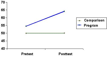
This design improves upon the posttest-only approach by measuring the dependent variable both before (pretest) and after (posttest) the intervention [1] [9]. The effect is inferred from the difference between these measurements. For instance, researchers might measure participants' weight before implementing a high-intensity training program, then measure again after three months of the intervention [1].

Methodological Considerations: Despite including a pretest, this design faces multiple threats to internal validity [1]. History effects (external events during the study), maturation (natural changes over time), testing effects (familiarity with measures), instrumentation changes (shifts in measurement tools), and regression to the mean (statistical tendency for extreme scores to move toward average) can all confound results [1] [9]. In biomedical contexts, spontaneous remission presents a particular challenge, as many medical conditions naturally improve over time without intervention [9].

Interrupted Time-Series Design

The interrupted time-series design strengthens the pretest-posttest approach by collecting multiple measurements both before and after the intervention [6] [9] [4]. This design tracks outcomes at regular intervals over an extended period, with the intervention introduced at a specific point. For example, a hospital might measure medication error rates monthly for a year before and after implementing a new electronic health record system [4].

Methodological Considerations: The multiple data points allow researchers to identify underlying trends and distinguish intervention effects from normal variability [9]. This design is particularly valuable for evaluating policy changes, public health initiatives, and system-wide interventions in biomedical settings [6] [4]. Statistical techniques such as segmented regression analysis are typically used to analyze time-series data.

Quasi-Experimental Designs: Multiple-Group Approaches

Multiple-group designs incorporate comparison groups that do not receive the intervention or receive a different intervention, substantially strengthening causal inference.

Nonequivalent Control Group Design

The nonequivalent control group design includes both an experimental group and a control group, but participants are not randomly assigned to these conditions [1] [10]. Groups are typically formed based on pre-existing characteristics or natural groupings. For example, researchers might study the effect of an app-based memory game by implementing it at one senior center (treatment group) while using another similar senior center as a control that continues usual activities [1].

Methodological Considerations: This design controls for many threats to internal validity, including history, maturation, testing, and regression to the mean, provided these factors affect both groups similarly [1]. The primary limitation is selection bias—the groups may differ systematically at baseline in ways that influence outcomes [1] [3]. Statistical techniques like analysis of covariance (ANCOVA) can adjust for pretest differences, while propensity score matching can create more comparable groups [8] [6].

Regression Discontinuity Design

Regression discontinuity design assigns participants to treatment and control groups based on a cutoff score on a pre-intervention measure [2] [6]. For example, students scoring below a certain threshold on a standardized test might receive remedial tutoring, while those above the threshold do not [6]. This approach comes closest to experimental design in methodological rigor [2].

Methodological Considerations: This design requires large sample sizes and precise modeling of the relationship between the assignment variable and outcome [2]. The key advantage is that it eliminates selection bias around the cutoff point, as assignment is determined solely by the predetermined threshold [6].

Difference-in-Differences Analysis

Difference-in-differences analysis compares changes in outcomes between treatment and control groups before and after an intervention [6]. This approach calculates the intervention effect as the difference in pre-post changes between groups. For example, this method was used to study the employment effects of minimum wage increases by comparing changes in employment between states that implemented increases and those that did not [6].

Methodological Considerations: This design controls for time-invariant confounders and selection bias related to fixed group differences [6]. It requires the parallel trends assumption—that in the absence of the intervention, both groups would have experienced similar changes over time.

Comparative Analysis: Single-Group vs. Multiple-Group Designs

Table: Comparison of Single-Group and Multiple-Group Quasi-Experimental Designs

Design Characteristic	Single-Group Designs	Multiple-Group Designs
Basic Structure	One group measured before/after intervention [9]	Two or more groups compared [1]
Control for History	No	Yes [1]
Control for Maturation	No	Yes [1]
Control for Testing Effects	No	Yes [1]
Control for Selection Bias	No	Partial [8]
Implementation Feasibility	High	Moderate
Causal Inference Strength	Weak	Moderate to Strong [1] [2]
Statistical Power	Lower (within-group comparisons)	Higher (between-group comparisons)
Primary Threats	History, maturation, testing, instrumentation, regression [9]	Selection bias, interaction of selection with other threats [1]

Applications in Biomedical Science

Healthcare Interventions and Policy Evaluation

Quasi-experimental designs are extensively used to evaluate healthcare interventions and policy changes where randomization is impractical or unethical [3] [4]. For example, researchers employed a quasi-experimental design to assess the effectiveness of a childhood obesity prevention program, finding that while the program reduced obesity risk, it was also expensive to implement [6]. Similarly, these designs have been used to evaluate the impact of electronic health record systems on medication errors, the effectiveness of hand hygiene interventions, and the outcomes of antimicrobial stewardship programs [3] [4].

Pharmaceutical and Clinical Research

In drug development and clinical research, quasi-experiments provide valuable evidence when RCTs cannot be conducted. For instance, comparing pregnancy outcomes in women who did versus did not receive antidepressant medication during pregnancy represents a classic quasi-experimental application in pharmacology, as random assignment would be unethical [8]. These designs are particularly valuable for studying rare diseases, special populations, or real-world medication effectiveness where traditional trials face recruitment challenges or ethical constraints.

Public Health and Epidemiology

Public health research frequently employs quasi-experimental designs to evaluate population-level interventions, such as the impact of public health policies, educational campaigns, or environmental changes [1] [4]. The interrupted time-series design has been used to study the effects of public smoking bans on cardiovascular events, the impact of vaccination programs on disease incidence, and the effectiveness of traffic safety laws on accident rates [6] [4].

Methodological Protocols and Statistical Considerations

Design and Implementation Protocols

Step 1: Design Selection

• Assess feasibility of random assignment [3]
• Identify available comparison groups or natural experiments [10]
• Determine appropriate pretest and posttest measures [1]
• Consider time-series approaches for longitudinal data [4]

Step 2: Sampling and Group Formation

• Implement matching techniques (individual, aggregate, or propensity score) to enhance group comparability [6] [10]
• Identify and measure potential confounding variables [8]
• Ensure adequate sample size through power analysis, accounting for anticipated effect sizes and potential clustering [6]

Step 3: Data Collection

• Standardize measurement procedures across groups [1]
• Implement blinding when possible to reduce ascertainment bias [4]
• Collect multiple pre-intervention and post-intervention measurements in time-series designs [9] [4]

Analytical Approaches

Multivariable regression represents the foundational analytical approach for quasi-experimental data, allowing researchers to adjust for measured confounding variables [8]. Propensity score matching creates statistical equivalence between groups by matching participants based on their probability of receiving the treatment [8] [6]. Instrumental variable analysis addresses unmeasured confounding by identifying variables that affect treatment assignment but not outcomes directly [6]. Segmented regression analyzes interrupted time-series data by modeling level and trend changes following interventions [4].

Research Reagent Solutions: Methodological Tools

Table: Essential Methodological Tools for Quasi-Experimental Research

Methodological Tool	Function	Application Context
Propensity Score Matching	Creates balanced treatment and control groups by matching on probability of treatment assignment [6]	Controls for selection bias when groups differ at baseline
Instrumental Variables	Addresses endogeneity (confounding) using variables related to treatment but not outcome [6]	Controls for unmeasured confounding when valid instruments available
Difference-in-Differences Analysis	Compares changes over time between treatment and control groups [6]	Evaluates policy interventions with longitudinal data
Regression Discontinuity	Exploits arbitrary cutoff points for treatment assignment [2] [6]	Studies interventions with eligibility thresholds
Multivariable Regression	Adjusts for confounding variables statistically [8]	Standard approach for most quasi-experimental analyses
Interrupted Time Series Analysis	Models intervention effects using multiple pre/post observations [9] [4]	Evaluates effects when single pre/post measures are insufficient

Quasi-experimental research designs occupy an essential niche in biomedical science, enabling causal inference when practical or ethical constraints preclude randomized experiments. While single-group designs offer implementation efficiency, multiple-group approaches provide substantially stronger evidence for causal relationships through comparison groups and advanced statistical adjustments. The rigorous application of these methodologies—including proper design selection, careful measurement, appropriate statistical analysis, and acknowledgment of limitations—allows biomedical researchers to generate valuable evidence for clinical practice, public health policy, and healthcare decision-making when traditional trials are not feasible. As methodological advancements continue to strengthen quasi-experimental approaches, their role in generating actionable evidence for complex biomedical questions will likely expand further.

Within the framework of a broader thesis on quasi-experimental research, understanding the distinction between single-group and multiple-group designs is paramount. This guide details the core methodological feature that separates these designs from true experiments: the absence of random assignment and the consequent challenges in establishing control [3]. In fields like drug development and public health, where randomized controlled trials (RCTs) are often impractical or unethical, quasi-experimental designs provide a critical alternative for evaluating causal relationships [1] [3]. These designs bridge the gap between observational studies and true experiments, allowing for investigation in real-world settings where researchers cannot control all influencing factors [1].

The following sections will dissect the role of randomization and control, compare specific quasi-experimental designs, and provide methodological guidance for applied researchers.

Fundamental Concepts: Randomization and Control

The Role of Randomization in Experimental Design

Randomization is the cornerstone of a true experiment. It refers to the process of randomly assigning study participants to either the treatment or control group [11] [12]. This procedure ensures that each participant has an equal chance of being placed in any group, thereby distributing both known and unknown confounding variables evenly across groups [13] [12]. The primary advantage of randomization is that it neutralizes systematic differences between groups at the outset of a study, allowing researchers to attribute any post-intervention differences in outcomes to the treatment itself [12].

The Concept of Control in Causal Inference

Control in research design serves as a benchmark for comparison. In a true experiment, the control group does not receive the intervention whose effect is being studied [13]. This group is essential for isolating the impact of the independent variable. Because of random assignment, the control group should be virtually identical to the treatment group in all respects except for the receipt of the intervention. Any difference in outcomes between these groups can then be more confidently inferred as the causal effect of the treatment [12].

How Quasi-Experiments Differ

Quasi-experimental designs are characterized by the lack of random assignment to treatment and control groups [11] [2]. In their place, researchers often use a comparison group, which is similar to a control group but is not formed through randomization [14]. This group may consist of units that are matched based on specific criteria or that naturally occur in the environment, such as students from a different school or patients from a different hospital [1] [14].

The critical limitation of this approach is selection bias [6]. Without randomization, there is no guarantee that the treatment and comparison groups are equivalent at baseline. Any observed differences in outcomes could therefore be due to these pre-existing differences rather than the intervention [3]. Consequently, while quasi-experiments can demonstrate that a relationship exists between an intervention and an outcome, they are less able to rule out alternative explanations, thus threatening the internal validity of the study [3] [15].

Table 1: Key Characteristics of True vs. Quasi-Experimental Designs

Feature	True Experiment	Quasi-Experiment
Random Assignment	Yes [11] [12]	No [11] [2]
Control Group	Yes, formed via randomization [13]	Uses a non-randomly assigned comparison group [14]
Primary Strength	High internal validity; strong causal inference [12]	High external validity; feasibility in real-world settings [1] [2]
Primary Limitation	Can be impractical or unethical; may lack external validity [3] [12]	Lower internal validity due to potential confounding [3] [15]
Context	Controlled laboratory or field settings [13]	Natural, real-world environments [1] [2]

Quasi-experimental designs can be broadly categorized into single-group and multiple-group designs, a distinction central to the overarching thesis of this research. This classification is based on whether the design incorporates an external group for comparison, which directly influences the strategy for establishing a counterfactual [16].

Single-Group Designs

Single-group designs are those in which all included units are exposed to the treatment [16]. The counterfactual is constructed using only data from the treated group itself, typically from time periods before the intervention.

• One-Group Pretest-Posttest Design: This common design involves measuring the dependent variable in a single group both before (pretest) and after (posttest) an intervention [1] [6]. The change from the pretest to the posttest is inferred to be the effect of the intervention. However, this design is highly susceptible to threats to internal validity, including:

  • History: External events occurring between the pretest and posttest that could affect the outcome [1] [3].
  • Maturation: Natural changes within participants over time, such as growth or fatigue, that could be mistaken for a treatment effect [1] [3].
  • Testing: The effect of taking the pretest on the scores of the posttest [3].
  • Regression to the Mean: The statistical phenomenon where subjects selected for their extreme scores (e.g., very high or very low) naturally tend to score closer to the average on subsequent measurements [1] [3].

• Interrupted Time-Series (ITS) Design: This design strengthens the one-group pretest-posttest by collecting multiple observations of the dependent variable both before and after the intervention [16] [15]. By analyzing the underlying trend before the intervention and seeing if the intervention "interrupts" this trend, researchers can make more robust causal claims. This design is particularly valuable for assessing the impact of policies or interventions at a population level [6].

Multiple-Group Designs

Multiple-group designs incorporate data from both a treated group and an untreated comparison group [16]. The use of a comparison group helps control for some of the threats to validity that plague single-group designs.

• Nonequivalent Groups Design (Pretest-Posttest with a Control Group): This design mimics a true experiment but without random assignment. It involves a treatment group and a control group, both of which are measured before and after the intervention [1] [14]. Any difference in the change between the pretest and posttest for the two groups is attributed to the intervention. While stronger than single-group designs, the core threat remains selection bias, as the groups may not be comparable at baseline [1].

• Difference-in-Differences (DID): This is a statistical technique used with nonequivalent group designs. It calculates the effect of an intervention by comparing the change in outcomes over time for the treatment group to the change in outcomes over time for the comparison group [6]. This method helps control for fixed differences between groups and for common trends over time [16].

• Regression Discontinuity Design (RDD): This is considered one of the most methodologically rigorous quasi-experimental designs [2]. Participants are assigned to the treatment or control group based on a cutoff score on a continuous variable (e.g., students below a certain test score receive remedial tutoring) [6] [15]. By comparing outcomes of individuals just on either side of the cutoff, researchers can estimate the causal effect of the treatment with high internal validity, as assignment is based solely on the predetermined cutoff [2].

Table 2: Comparison of Single-Group and Multiple-Group Quasi-Experimental Designs

Design Feature	Single-Group Designs	Multiple-Group Designs
Definition	All included units receive the treatment; no external control group [16].	Includes both treated and untreated groups for comparison [16].
Core Counterfactual	The group's own pre-intervention state [16].	An external, untreated comparison group [16].
Key Threats to Validity	History, Maturation, Testing, Instrumentation [1] [3].	Selection Bias, Differential Attrition [1] [3].
Data Requirements	Pre- and post-intervention data for the treated unit(s) [16].	Pre- and post-intervention data for both treated and comparison units [16].
Relative Strength	Useful when no comparable control group is available [16].	Provides better control for external events (history) and maturation [1].
Examples	One-Group Pretest-Posttest, Interrupted Time Series [1] [16].	Nonequivalent Control Group, Difference-in-Differences, Regression Discontinuity [1] [6].

Methodological Protocols and Statistical Control

When random assignment is not possible, researchers must employ rigorous methodological protocols and statistical techniques to strengthen the validity of their quasi-experimental studies.

Design-Based Control Methods

• Matching: This technique involves pairing each participant in the treatment group with one or more participants from a potential comparison pool who are similar on key pre-intervention characteristics (e.g., age, disease severity, socioeconomic status) [14]. This creates a comparison group that is more analogous to the treatment group at baseline.

  • Propensity Score Matching (PSM): A popular matching method where a statistical model predicts the probability (propensity) of each unit receiving the treatment, given its observed covariates. Treatment and control units are then matched based on these scores, simulating the condition of randomization [6].

• Instrumental Variables (IV): An instrumental variable is one that is correlated with the independent variable but does not have a direct effect on the dependent variable, except through its correlation with the independent variable [6]. If a valid instrument can be found, it can be used to isolate the part of the independent variable that is not correlated with the error term, thus addressing unmeasured confounding [6].

Analytical Workflows for Causal Inference

The following diagram illustrates a generalized analytical workflow for a quasi-experimental study, highlighting key decision points for mitigating bias.

Diagram 1: Quasi-Experimental Analysis Workflow

The Researcher's Toolkit: Essential Methodological Solutions

For researchers employing quasi-experimental designs, the "toolkit" consists not of physical reagents but of methodological and statistical solutions to address the inherent challenge of confounding.

Table 3: Essential Methodological Solutions for Quasi-Experimental Research

Tool	Primary Function	Key Considerations
Propensity Score Matching	To create a comparison group that is statistically similar to the treatment group by matching on the probability of receiving treatment [6].	Computationally complex; sensitive to the choice of matching algorithm; cannot control for unobserved confounding [6].
Difference-in-Differences (DID)	To control for pre-existing, time-invariant differences between groups and common temporal trends by comparing the change in outcomes [16] [6].	Relies on the "parallel trends" assumption; can be confounded by events that affect groups differently during the study period [16] [6].
Instrumental Variables (IV)	To address unmeasured confounding by using a variable that influences the treatment but affects the outcome only through the treatment [6].	Finding a valid instrument is very difficult; instruments must be strongly correlated with the treatment and satisfy exclusion restrictions [6].
Regression Discontinuity	To estimate causal effects by comparing units on either side of a predetermined assignment cutoff [6] [2].	Requires a large sample size near the cutoff; results are only directly generalizable to units close to the cutoff [2].
Sensitivity Analysis	To test how robust the study's conclusions are to potential unmeasured confounding [3].	Does not eliminate bias but quantifies how much hidden bias would be needed to alter the study's conclusions [3].

Quasi-experimental designs are indispensable in the researcher's arsenal for situations where RCTs are not a viable option. The fundamental distinction from true experiments lies in the absence of randomization, which is replaced by various design and statistical methods to approximate a counterfactual. The choice between single-group and multiple-group designs, a central theme of this research, involves a direct trade-off between feasibility and validity. Single-group designs are applicable when no comparison group exists but are vulnerable to many threats. Multiple-group designs offer greater internal validity but require the identification of a suitable comparison group and rigorous methods like matching or DID to mitigate selection bias. By carefully selecting the appropriate design and applying robust methodological tools, researchers in drug development, public health, and policy can derive causally plausible and impactful evidence from real-world data.

In scientific research, particularly in fields where randomized controlled trials are not feasible for ethical or practical reasons, quasi-experimental designs provide a critical methodological foundation. These designs attempt to establish cause-and-effect relationships between an independent and dependent variable, but unlike true experiments, they do not rely on random assignment of subjects to groups [17]. Instead, participants are assigned to groups based on non-random criteria, such as existing characteristics, geographical location, or timing of an intervention [17]. This paper explores the spectrum of quasi-experimental approaches, focusing on the comparative strengths and limitations of single-group and multiple-group designs within the context of applied research settings, including drug development and public health evaluation.

Quasi-experimental designs occupy a middle ground on the control continuum—offering more rigor than pre-experimental designs but less than true experimental designs [18]. They are particularly valuable when researchers need to evaluate real-world interventions that cannot be administered in laboratory settings or when withholding treatment for control purposes would be unethical [1] [17]. For instance, studying the effects of a new health policy or the impact of a natural disaster on community health outcomes typically necessitates quasi-experimental approaches because random assignment is impossible [1] [10].

Core Concepts and Terminology

Understanding quasi-experimental research requires familiarity with several key concepts:

• Independent Variable (IV): The treatment, intervention, or condition manipulated or studied for its effects on outcomes [18]. In quasi-experiments, researchers often do not have direct control over this variable [17].
• Dependent Variable (DV): The outcome measure that is hypothesized to be influenced by the independent variable [18].
• Internal Validity: The degree to which a cause-and-effect relationship between variables can be established without interference from other factors [1]. Threats to internal validity are a primary concern in quasi-experimental designs.
• External Validity: The generalizability of research results beyond the study context [1].
• Control Group: A group that does not receive the experimental treatment, used for comparison purposes [17]. In quasi-experiments, this is often called a "comparison group" since assignment is not random [10].
• Confounding Variables: Extraneous factors that may inadvertently influence the dependent variable, creating misleading interpretations about cause-and-effect relationships [1].

Single-Group Quasi-Experimental Designs

Single-group designs involve studying one group of participants who receive an intervention or treatment. These approaches are generally considered weaker than multiple-group designs but are necessary when comparison groups are unavailable or unethical to implement.

One-Group Posttest Only Design

The one-group posttest only design represents the simplest quasi-experimental approach. Researchers implement a treatment and then measure the dependent variable once after the treatment is completed [9]. For example, a researcher might implement an anti-drug education program and then immediately measure students' attitudes toward illegal drugs [9].

Key Limitations: This is considered the weakest type of quasi-experimental design due to the complete absence of both a control group and a pretest [9]. Without a comparison point, it is impossible to determine what participants' attitudes or behaviors would have been without the intervention. Results from such designs are frequently reported in media and often misinterpreted by the general public [9].

One-Group Pretest-Posttest Design

In the one-group pretest-posttest design, researchers measure the dependent variable once before implementing the treatment and once after implementation [9] [1]. This approach is similar to a within-subjects experiment where each participant is tested under both control and treatment conditions, though without counterbalancing [9].

This design improves upon the posttest-only approach by providing a baseline measurement, but it remains vulnerable to several threats to internal validity [9] [1]:

• History: External events between pretest and posttest may influence outcomes.
• Maturation: Natural changes in participants over time may affect results.
• Testing: Exposure to the pretest may influence posttest performance.
• Instrumentation: Changes in measurement tools or procedures may create apparent effects.
• Regression to the Mean: Extreme scores on the pretest may naturally move toward average on the posttest.
• Spontaneous Remission: Natural improvement over time without treatment.

Table 1: Threats to Internal Validity in One-Group Pretest-Posttest Designs

Threat Type	Description	Example
History	External events between pretest and posttest influence outcomes	A celebrity drug overdose occurs during an anti-drug program [9]
Maturation	Natural developmental changes affect results	Participants become less impulsive with age during a year-long program [9]
Testing	Taking the pretest influences posttest performance	Completing a drug attitude survey prompts reflection that changes attitudes [9]
Instrumentation	Changes in measurement tools or procedures affect scores	Observers become more skilled or fatigued over time [9]
Regression to the Mean	Extreme pretest scores naturally move toward average	Students with extremely high drug attitudes scores show lower scores at posttest without program effect [9]
Spontaneous Remission	Natural improvement over time without treatment	Depression symptoms improve without therapeutic intervention [9]

Interrupted Time Series Design

A more robust single-group approach is the interrupted time series design, which involves multiple measurements of the dependent variable both before and after an intervention [9] [10]. This design strengthens inference by establishing trends before the intervention and tracking persistence of effects afterward [9].

For example, a researcher might measure student absences per week for several weeks, implement an attendance-tracking intervention, then continue measuring absences for several more weeks [9]. If an immediate and sustained drop in absences follows the intervention, this provides stronger evidence for treatment effect than a simple pretest-posttest design [9]. The multiple measurement points help distinguish true treatment effects from normal variability [9].

Diagram 1: Interrupted Time Series Design

Multiple-Group Quasi-Experimental Designs

Multiple-group designs provide stronger evidence for causal relationships by including comparison groups that do not receive the experimental treatment or receive different versions of it.

Nonequivalent Groups Design

The nonequivalent groups design is the most common multiple-group quasi-experimental approach [17]. Researchers select existing groups that appear similar, with only one group receiving the treatment [17] [10]. The critical limitation is that without random assignment, the groups may differ in important ways—they are "nonequivalent" [17] [10].

For example, a researcher might study the effect of an app-based memory game on cognitive function by recruiting older adults from two similar senior centers [1]. One center receives the game intervention, while the other continues with usual activities. Both groups complete memory tests before and after the intervention period [1]. Any differences in posttest scores between the groups, assuming similar pretest scores, might be attributed to the intervention [1].

Posttest-Only Design with Control Group

This design includes both an experimental group that receives an intervention and a control group that does not, with both groups measured only after the intervention [1]. For instance, researchers might implement a new hand hygiene intervention at one hospital but not at a similar hospital, then compare infection rates after three months [1].

Key Limitations: The absence of pretest measurements makes it impossible to determine if groups were equivalent before the intervention [1]. Observed differences in posttest measures could result from either the intervention or pre-existing differences between groups [1].

Pretest-Posttest Design with Control Group

This stronger multiple-group design includes pretest measurements for both treatment and control groups before the intervention, followed by posttest measurements after [1]. Similar pretest scores between groups increase confidence that any posttest differences result from the intervention [1].

Despite being one of the strongest quasi-experimental designs, it remains vulnerable to threats, particularly selection biases and differential history effects [1]. If participants are not randomized, unmeasured confounding variables might explain observed effects [1]. Additionally, external events might differentially affect the treatment and control groups between pretest and posttest measurements [1].

Diagram 2: Pretest-Posttest Design with Control Group

Comparative Analysis: Single-Group vs. Multiple-Group Designs

The choice between single-group and multiple-group designs involves trade-offs between practical feasibility and scientific rigor. The table below summarizes key comparative aspects:

Table 2: Comparison of Single-Group and Multiple-Group Quasi-Experimental Designs

Design Characteristic	Single-Group Designs	Multiple-Group Designs
Control Requirements	Minimal control needed; suitable when only one group is accessible [9]	Requires access to multiple comparable groups [1]
Internal Validity	Lower; vulnerable to history, maturation, testing, instrumentation, regression to the mean [9]	Higher; controls for several threats through comparison groups [1]
External Validity	Potentially higher for the specific population studied [17]	May be limited if groups are not representative [1]
Implementation Practicality	Generally more practical and cost-effective [9]	More complex and resource-intensive [19]
Statistical Power	Limited without comparison group [9]	Enhanced through between-group comparisons [20]
Causal Inference Strength	Weak; cannot rule out many alternative explanations [9]	Moderate; can rule out some alternative explanations [1]
Common Applications	Preliminary studies, program evaluations with limited resources [9]	Policy evaluations, comparative effectiveness research [1] [17]

Methodological Considerations and Best Practices

Enhancing Internal Validity in Quasi-Experimental Designs

Researchers can employ several strategies to strengthen quasi-experimental designs:

• Matching Techniques: When random assignment is impossible, researchers can match participants between treatment and control groups based on key demographic or clinical variables [10]. Individual matching pairs participants with similar attributes, then splits the pair between groups [10]. Aggregate matching ensures the overall comparison group is similar to the treatment group on important variables [10].

• Statistical Control: Advanced statistical methods can adjust for pre-existing differences between groups, though this cannot completely compensate for lack of randomization [1].

• Multiple Pretest Measurements: Collecting several baseline measurements helps establish trends and account for normal variability before intervention [9].

• Careful Selection of Comparison Groups: Choosing comparison groups from similar settings (e.g., same hospital system, similar communities) reduces confounding [1] [10].

Analytical Approaches for Multiple-Group Designs

When analyzing data from multiple-group designs, researchers must select appropriate statistical methods:

• Multiple Comparison Procedures: When comparing more than two groups, researchers must account for increased Type I error rates using specialized procedures [20]:

  • Tukey's HSD: Most powerful test for all pairwise comparisons [20]
  • Dunnett's Test: Optimal when comparing multiple treatment groups to a single control [20]
  • Games-Howell Procedure: Appropriate when groups have unequal variances [20]

• Handling Overlapping Group Membership: When participants belong to multiple groups, standard ANOVA becomes problematic, and pairwise comparison methods with appropriate corrections are recommended [21].

Applications in Drug Development and Public Health Research

Quasi-experimental designs have particular relevance in pharmaceutical and public health research where randomized trials may be impractical or unethical.

Natural Experiments in Health Policy Research

Natural experiments occur when comparable groups are created by real-world differences rather than researcher manipulation [17] [10]. The Oregon Health Study represents a classic example, where a lottery system for Medicaid enrollment created natural treatment and control groups for studying health insurance effects [17]. Such approaches enable research on important policy questions that could not be studied through randomized designs for ethical reasons [17].

Interrupted Time Series in Medication Adherence Studies

Time series designs can evaluate the impact of new medications or adherence interventions by examining trends in health outcomes before and after implementation [9]. For instance, researchers might analyze hospital admission rates for heart failure patients before and after introducing a new medication management program, using multiple data points to establish causal inference [9].

Essential Research Reagents and Materials

Table 3: Key Research Reagent Solutions for Quasi-Experimental Studies

Research Component	Function/Application	Implementation Example
Validated Assessment Tools	Standardized measurement of dependent variables	Memory tests in cognitive intervention studies [1]
Data Collection Platforms	Efficient gathering of pretest/posttest data	Electronic survey systems for patient-reported outcomes [1]
Statistical Software with Multiple Comparison Capabilities	Appropriate analysis of group differences	Software implementing Tukey, Dunnett, and Games-Howell procedures [20]
TREND Statement Guidelines	Reporting standards for nonrandomized designs	22-item checklist for transparent reporting of quasi-experimental studies [1]
Matching Algorithms	Creating comparable treatment and control groups	Procedures for individual or aggregate matching on prognostic variables [10]

The spectrum from single-group to multiple-group quasi-experimental designs offers researchers a range of methodological options for studying causal relationships when randomized trials are not feasible. Single-group designs, including posttest-only, pretest-posttest, and interrupted time series approaches, provide practical solutions for preliminary investigations and situations with limited resource availability, though they suffer from significant threats to internal validity. Multiple-group designs, particularly nonequivalent group designs with pretest and posttest measurements, offer stronger causal inference through comparison groups, though they require greater resources and remain vulnerable to selection biases.

The choice between these approaches should be guided by research questions, practical constraints, and ethical considerations. While multiple-group designs generally provide more rigorous evidence, well-executed single-group designs—particularly interrupted time series—can yield valuable insights when enhanced with multiple measurement points and careful attention to threats to internal validity. As quasi-experimental methodologies continue to evolve, they remain indispensable tools for researchers addressing critical questions in drug development, public health, and social policy.

Independent and Dependent Variables in Quasi-Experimental Contexts

Quasi-experimental designs are research methodologies used to estimate causal relationships when true experimental controls are not feasible [15]. These designs occupy a crucial space between observational studies and true experiments, sharing similarities with randomized controlled trials but specifically lacking random assignment to treatment or control groups [2]. Instead, assignment to treatment condition typically proceeds as it would naturally occur in the absence of an experiment [2]. The fundamental purpose of quasi-experimental research is to investigate cause-and-effect relationships between variables in real-world settings where researchers cannot employ traditional experimental methods due to ethical constraints, practical limitations, or resource restrictions [22].

In these designs, researchers actively study the effects of independent variables on dependent variables without full experimental control [22]. This approach is particularly valuable in social sciences, public health, education, and policy analysis where manipulating variables or randomly assigning participants could be unethical or impractical [2]. For example, studying the health effects of a natural disaster or evaluating the impact of a new public policy often necessitates quasi-experimental approaches because researchers cannot control who receives the "treatment" (e.g., who experiences the disaster or is affected by the policy) [1] [17].

Core Components: Independent and Dependent Variables

Independent Variables in Quasi-Experiments

In quasi-experimental research, the independent variable (IV) is the factor or condition that researchers aim to study, though they often cannot manipulate it directly as in true experiments [22]. Unlike controlled experiments where investigators deliberately manipulate the IV, quasi-experimental designs frequently deal with naturally occurring variables or pre-existing conditions [2] [22]. These are sometimes termed "quasi-independent" variables because they lack the controlled manipulation characteristic of true experiments [15].

Examples of independent variables in quasi-experimental contexts include:

• Naturally occurring events: Natural disasters, policy changes, or public health interventions [1] [17]
• Pre-existing group characteristics: Age, gender, diagnostic status, or institutional affiliation [2] [15]
• Program participation: Enrollment in an educational intervention, exposure to a training program, or receipt of a social benefit [10] [23]

A key characteristic of independent variables in quasi-experiments is that their "levels" or variations occur without researcher intervention. For instance, in studying the health impacts of a hurricane, the independent variable (hurricane exposure) occurs naturally, and researchers simply identify groups with different exposure levels [1].

Dependent Variables in Quasi-Experiments

The dependent variable (DV) represents the outcome or response that researchers measure to assess the effects of changes in the independent variable [22]. These variables capture the anticipated effects or consequences of the quasi-independent variable and are measured through quantitative data collection methods [15].

Examples of dependent variables in quasi-experimental research include:

• Behavioral measures: Healthcare utilization rates, academic performance, or employment outcomes [1] [24]
• Psychological indicators: Stress levels, attitudes, or cognitive test scores [1] [9]
• Physiological measures: Blood pressure, infection rates, or mortality statistics [1]
• System-level outcomes: Organizational productivity, public health statistics, or economic indicators [23]

The dependent variable must be precisely defined and reliably measured, as the validity of causal inferences depends on accurately detecting changes that might be attributed to the independent variable [1] [22].

Table 1: Characteristics of Variables in Quasi-Experimental Designs

Variable Type	Definition	Researcher Control	Examples
Independent Variable	The presumed cause or intervention being studied	Limited or none; often naturally occurring or pre-existing	Policy changes, natural disasters, pre-existing group characteristics [1] [2] [22]
Dependent Variable	The outcome measured to assess intervention effects	Direct control over measurement but not the outcome itself	Test scores, health outcomes, behavioral observations [1] [22]
Quasi-Independent Variable	A specific type of independent variable using inherent characteristics	None; characteristics are inherent to participants	Eye color, diagnostic status, age, gender [15]

Quasi-Experimental Design Typologies

Single-Group Quasi-Experimental Designs

Single-group designs involve studying one group of participants who receive an intervention or are exposed to a condition, with measurements taken to assess potential effects [9]. These designs are particularly useful when no comparable control group is available, though they present significant challenges for establishing causal inference [9] [24].

One-Group Posttest-Only Design is the simplest form of quasi-experimental design [9] [10]. In this approach, a single group is exposed to the independent variable, and data on the dependent variable is collected only after the intervention [9] [22]. For example, researchers might implement a new teaching method and then measure student performance immediately afterward [9]. The major limitation of this design is the absence of both a control group and a pretest, making it difficult to determine what outcomes would have occurred without the intervention [9] [10].

One-Group Pretest-Posttest Design extends the previous approach by including a measurement of the dependent variable before the intervention [1] [9] [10]. Participants are measured on the dependent variable (pretest), exposed to the independent variable, and then measured again (posttest) [1] [9]. The effect of the intervention is inferred from differences between pretest and posttest results [1]. For example, researchers might measure weight loss program participants before and after a three-month high-intensity training intervention [1]. Despite the inclusion of a pretest, this design remains vulnerable to multiple threats to internal validity, including history effects, maturation, testing effects, instrumentation, and regression to the mean [1] [9] [23].

Interrupted Time-Series Design incorporates multiple observations of the dependent variable both before and after the implementation of the independent variable [9] [10] [24]. This approach involves collecting data at regular intervals before the intervention to establish a baseline trend, then continuing data collection after the intervention to observe any changes in that trend [9] [23]. For example, a manufacturing company might measure worker productivity weekly for a year, implement a change in work shift length, and continue measuring productivity to assess the intervention's impact [9] [23]. This design strengthens causal inference by demonstrating whether changes persist beyond normal variability [9] [23].

Multiple-Group Quasi-Experimental Designs

Multiple-group designs incorporate comparison groups that do not receive the experimental intervention, providing valuable reference points for interpreting results [1] [17] [10].

Nonequivalent Groups Design (also called pretest-posttest with control group design) involves selecting groups that appear similar but where only one receives the treatment [1] [17] [23]. The researcher selects a group to receive the treatment and another with similar characteristics to serve as the control group [1] [10]. Both groups complete a pretest, after which the treatment group receives the intervention, and finally, both groups complete a posttest [1] [23]. For example, in a study examining memory improvement in older adults, participants from one senior center might use an app-based game while those from another similar center engage in usual activities, with both groups completing memory tests before and after the intervention period [1]. The primary limitation is that without random assignment, the groups may differ in important ways that affect the outcome [1] [17] [23].

Posttest-Only Design with Nonequivalent Groups uses two groups—an experimental group that receives an intervention and a control group that does not—with measurements taken only after the intervention [1] [25]. For example, researchers might compare infection rates between two similar hospitals after implementing a new hand hygiene protocol at only one facility [1]. This design does not include pretest measurements, making it difficult to determine if groups were comparable before the intervention [1] [25].

Regression Discontinuity Design assigns participants to treatment conditions based on a specific cutoff score on a predetermined measure [17] [22] [15]. Those just above and below the cutoff are considered comparable, allowing for causal inference about the treatment's effect [17] [15]. For example, students scoring just below a proficiency threshold might receive additional tutoring while those just above do not, with subsequent academic performance compared between groups [17] [22]. This design provides strong causal evidence when implemented properly [2].

Methodological Considerations and Protocols

Implementation Protocols for Key Designs

Protocol for One-Group Pretest-Posttest Design

• Participant Selection: Identify participants based on convenience and suitability for the study [1]. Develop specific eligibility criteria related to the research question [1].
• Pretest Administration: Measure the dependent variable before implementing the intervention [1] [9]. Ensure measurement tools are valid and reliable for the construct being assessed [1].
• Intervention Implementation: Expose participants to the independent variable under controlled conditions when possible [1]. Document intervention details thoroughly for replication.
• Posttest Administration: Measure the dependent variable again after the intervention using the same protocol as the pretest [1] [9].
• Data Analysis: Compare pretest and posttest scores using appropriate statistical tests (e.g., paired t-tests) [1]. Calculate effect sizes to determine practical significance.

Protocol for Nonequivalent Groups Design

• Group Selection: Identify existing groups that appear similar in relevant characteristics [1] [17] [23]. Select one group to receive the treatment and another to serve as the control [1].
• Pretest Administration: Measure the dependent variable in both groups before the intervention [1] [23]. Collect demographic and other potentially confounding variables to assess group similarity [1].
• Treatment Implementation: Implement the intervention in the treatment group only [1]. The control group continues with standard conditions or receives an alternative intervention [1] [17].
• Posttest Administration: Measure the dependent variable in both groups after the intervention period [1] [23].
• Data Analysis: Test for pretest similarity between groups [1]. Analyze posttest scores using statistical methods that control for pretest differences (e.g., ANCOVA) [1] [23]. Examine whether demographic variables need statistical control [1].

Protocol for Interrupted Time-Series Design

• Baseline Establishment: Collect multiple measurements of the dependent variable at regular intervals before the intervention [9] [23]. Ensure sufficient data points to establish a stable trend (typically at least 5-10 observations) [9].
• Intervention Implementation: Introduce the independent variable at a clearly defined point in time [9] [23].
• Post-Intervention Monitoring: Continue collecting measurements at the same intervals after the intervention [9] [23]. Maintain data collection long enough to detect sustained effects.
• Data Analysis: Use time-series analysis techniques to determine if the intervention caused a change in the level or trend of the dependent variable beyond what would be expected based on pre-intervention patterns [9] [23].

Threats to Validity and Mitigation Strategies

Quasi-experimental designs face significant threats to internal validity—the approximate truth about inferences regarding cause-effect relationships [2] [22]. Understanding these threats is essential for designing robust studies and interpreting results appropriately.

Table 2: Threats to Internal Validity in Quasi-Experimental Designs

Threat	Description	Most Vulnerable Designs	Mitigation Strategies
History	External events between pretest and posttest that influence outcomes [1] [9] [23]	One-group pretest-posttest [1] [9]	Include comparison groups; use time-series with multiple measurements [9] [10]
Maturation	Natural changes in participants over time that affect results [1] [9] [23]	One-group pretest-posttest [1] [9]	Include control groups; statistical controls [1] [23]
Selection Bias	Systematic differences between groups at baseline due to non-random assignment [1] [17] [22]	All multiple-group designs [1] [17]	Careful group matching; statistical controls; propensity score matching [10] [22]
Regression to Mean	Extreme scores tending toward average on retesting [1] [9] [23]	Designs selecting participants based on extreme scores [1] [9]	Use comparison groups; avoid selecting based on extreme scores [9] [23]
Testing Effects	Changes in scores due to familiarity with measures [9]	Pretest-posttest designs [9]	Use different but equivalent forms; include comparison groups [9]
Instrumentation	Changes in measurement tools or procedures over time [9]	Time-series; pretest-posttest [9]	Standardize measurement procedures; calibrate instruments [9]

Table 3: Research Reagent Solutions for Quasi-Experimental Research

Research Tool	Function	Application Context
TREND Guidelines	22-item checklist for transparent reporting of nonrandomized designs [1]	Improving reporting quality and methodological rigor [1]
Propensity Score Matching	Statistical technique to create comparable treatment and control groups by matching on predicted probability of group membership [22]	Balancing groups on observed covariates in nonrandomized studies [22]
Statistical Control Methods	Techniques like regression analysis to statistically adjust for group differences [2] [25]	Accounting for confounding variables in analysis phase [2]
Standardized Measurement Instruments	Validated tools for assessing dependent variables [1]	Ensuring reliable and valid outcome measurement across groups and time [1]
Time-Series Analysis	Statistical methods for analyzing data collected at regular intervals over time [9] [23]	Identifying trends and intervention effects in time-series designs [9] [23]

Comparative Analysis and Design Selection

Comparative Strengths and Limitations

The choice between single-group and multiple-group quasi-experimental designs involves trade-offs between practical feasibility and scientific rigor. Single-group designs are typically easier to implement, require fewer participants, and are more feasible when suitable comparison groups cannot be identified [9] [10]. However, they suffer from significant limitations in establishing causal relationships due to the inability to rule out many threats to internal validity [1] [9].

Multiple-group designs provide stronger evidence for causal inference by offering a reference point for comparing outcomes [1] [17]. The inclusion of comparison groups helps researchers account for external events, maturation effects, and other threats that might otherwise be attributed to the intervention [1] [23]. However, these designs require identifying appropriate comparison groups and managing potential selection biases [17] [23].

Table 4: Comparative Analysis of Quasi-Experimental Designs

Design Type	Internal Validity	External Validity	Implementation Practicality	Causal Inference Strength
One-Group Posttest-Only	Very Low [9] [10]	Moderate [9]	High [9]	Very Weak [9] [10]
One-Group Pretest-Posttest	Low [1] [9]	Moderate [1]	High [1]	Weak [1] [9]
Interrupted Time-Series	Moderate-High [9] [23]	High [9]	Moderate [9]	Moderate [9] [23]
Nonequivalent Groups	Moderate [1] [17]	High [17]	Moderate [1]	Moderate [1] [17]
Regression Discontinuity	High [2] [15]	Limited to cutoff area [17]	Moderate [17]	Strong [2] [15]

Design Selection Framework

Selecting an appropriate quasi-experimental design requires careful consideration of research questions, practical constraints, and ethical considerations. The following decision framework can guide researchers:

• Assess Feasibility of Comparison Groups: If suitable comparison groups are available, multiple-group designs are generally preferred for their stronger causal inference capabilities [1] [17]. When comparison groups cannot be identified, single-group designs may be the only option, though researchers should strengthen them through multiple pretest and posttest measurements when possible [9] [10].

• Consider Measurement Opportunities: When only post-intervention measurement is possible, posttest-only designs may be necessary despite their limitations [1] [9]. When both pre- and post-intervention measurements are feasible, pretest-posttest designs provide valuable baseline data [1] [9]. When resources allow for multiple measurements over time, time-series designs offer stronger causal evidence [9] [23].

• Evaluate Assignment Mechanisms: When participants are naturally assigned to conditions based on a cutoff score, regression discontinuity designs provide particularly strong causal evidence [17] [2] [15]. When groups are formed through self-selection or administrative processes, nonequivalent group designs with careful matching are appropriate [17] [10].

• Balance Practical and Scientific Considerations: While more complex designs generally offer stronger causal inference, they also require greater resources and methodological expertise [22]. Researchers must balance scientific ideals with practical constraints when selecting designs [17] [22].

Quasi-experimental designs provide essential methodological approaches for investigating causal relationships when randomized experiments are not feasible or ethical [1] [17]. These designs span a continuum from single-group approaches, which offer practical advantages but limited causal inference, to multiple-group designs that provide stronger evidence for causal relationships while requiring more complex implementation [1] [9] [17].

The core components of any quasi-experimental study are the independent variable (the presumed cause or intervention) and the dependent variable (the measured outcome) [22]. The relationship between these variables is investigated under naturalistic conditions where researchers lack full control over assignment to treatment conditions [2] [22]. This fundamental characteristic distinguishes quasi-experiments from true experiments and introduces unique methodological challenges, particularly regarding internal validity [2] [22].

When implementing quasi-experimental research, careful design selection is crucial [17] [22]. Researchers must balance practical constraints with methodological rigor, selecting designs that maximize causal inference within the limitations of their research context [17] [22]. Additionally, comprehensive reporting using guidelines like TREND enhances transparency and allows consumers of research to properly evaluate findings [1]. Through thoughtful application of these principles, quasi-experimental designs continue to make valuable contributions to knowledge across diverse fields of inquiry [1] [15].

Quasi-experimental designs (QEDs) represent a critical class of research methodologies employed when randomized controlled trials (RCTs) are not feasible or ethical. These designs enable researchers to estimate causal effects in real-world settings where random assignment is impractical. This technical guide provides an in-depth examination of the ethical and practical rationales for selecting QEDs, framed within the context of a broader thesis comparing single-group and multiple-group approaches. Aimed at researchers, scientists, and drug development professionals, the article synthesizes current methodological frameworks, presents structured comparisons of design features, and outlines detailed experimental protocols. Through standardized data presentation and visual workflows, we aim to equip practitioners with the necessary tools to implement rigorous quasi-experimental research in applied settings, particularly where ethical constraints or practical limitations preclude randomized designs.

Quasi-experimental design is a research methodology that occupies the strategic space between the rigorous control of true experimental designs and the observational nature of non-experimental studies [1]. These designs aim to establish cause-and-effect relationships but lack the random assignment to treatment and control groups that characterizes randomized controlled trials (RCTs) [2] [17]. The fundamental characteristic of QEDs is that assignment to treatment conditions occurs through non-random mechanisms, often through self-selection, administrative decisions, or natural circumstances [5]. This key difference makes QEDs particularly valuable for research questions where randomization is impossible or unethical, while still allowing for stronger causal inferences than purely observational approaches.

The conceptual foundation of QEDs rests on their ability to approximate the counterfactual logic of experimental design through methodological creativity rather than random assignment [26]. In a true experiment, random assignment ensures that, on average, treatment and control groups are equivalent in both observed and unobserved characteristics, allowing any post-intervention differences to be attributed to the treatment [2]. QEDs, by contrast, must address potential selection bias and confounding through design features such as pre-test measurements, multiple comparison groups, or statistical controls [1] [27]. This methodological approach enables researchers to draw reasonable causal inferences when practical or ethical constraints prevent randomization.

Within the research methodology hierarchy, QEDs are characterized by several key features: they manipulate an independent variable, measure a dependent variable, but lack random assignment [17]. They typically employ comparison groups rather than true control groups, with these groups often being "nonequivalent" due to the absence of randomization [28]. The internal validity of QEDs—the confidence that observed effects are truly caused by the intervention—is generally lower than in true experiments, but their external validity—the generalizability to real-world settings—is often higher [5] [17]. This tradeoff positions QEDs as particularly valuable for evaluating interventions in authentic contexts where perfect laboratory control is neither possible nor desirable.

Table 1: Fundamental Characteristics of Quasi-Experimental Designs

Characteristic	True Experiments	Quasi-Experiments	Observational Studies
Assignment Mechanism	Random assignment	Non-random assignment	No assignment
Control Over Treatment	Researcher-controlled	Often studies pre-existing treatments	No researcher control
Control Groups	Required	Not required but commonly used	Not applicable
Internal Validity	High	Moderate	Low
External Validity	Often lower	Higher	Highest
Primary Use Case	Efficacy under controlled conditions	Effectiveness in real-world settings	Identifying associations

Ethical and Practical Rationales for Selection

Ethical Rationales

Ethical considerations frequently necessitate the use of quasi-experimental designs when randomized assignment would be morally questionable or directly harmful. In healthcare research, it is often ethically impermissible to withhold standard treatment or proven interventions from patients solely for research purposes [27]. For instance, studying the effect of a new surgical technique alongside a base treatment would be unethical if researchers created a control group that received no treatment at all, as leaving patients without care violates fundamental medical ethics [27]. Similarly, in public health policy evaluation, randomly providing interventions such as health insurance to some while deliberately withholding it from others would be ethically problematic, as demonstrated by the Oregon Health Study, which instead leveraged a natural lottery system to study coverage effects [17].

Ethical constraints also emerge when studying vulnerable populations or sensitive behaviors where random assignment could cause harm or infringe upon rights [2]. Research on topics such as child discipline practices (e.g., spanking effects) cannot randomly assign parents to implement potentially harmful behaviors, making quasi-experimental approaches that leverage existing differences the only ethically viable option [2]. Likewise, in educational settings, deliberately withholding beneficial programs from students for research purposes typically violates ethical standards, leading researchers to use quasi-experimental comparisons between naturally occurring groups [1]. These ethical imperatives make QEDs not merely a methodological alternative but an ethical necessity across many research domains.

Practical Rationales

Practical constraints constitute the second major rationale for selecting quasi-experimental designs, occurring when randomization is theoretically possible but practically unfeasible. Financial limitations often preclude true experiments, as RCTs typically require substantial funding for participant recruitment, implementation of interventions, and management of control conditions [17] [26]. QEDs can frequently leverage existing data sources and naturally occurring interventions, significantly reducing research costs [17]. Logistical challenges also favor quasi-experimental approaches, particularly when studying interventions at organizational, community, or policy levels where random assignment is administratively impossible [1]. For example, evaluating the impact of a new law or large-scale public health initiative typically requires quasi-experimental methods because researchers cannot randomly assign jurisdictions to implement different policies [26].

Practical feasibility issues also arise when researchers lack authority to control treatment assignment, such as when studying existing organizational practices, policy changes, or medical treatments determined by clinicians rather than researchers [17] [27]. In these situations, methodological flexibility becomes essential, with QEDs allowing researchers to study important questions that cannot be answered through true experiments. Additionally, timeline constraints often favor quasi-experimental approaches, as they can frequently be implemented more quickly than RCTs, which require extensive planning for randomization procedures and control condition management [5]. This practical advantage makes QEDs particularly valuable for rapidly evaluating emerging public health threats or policy responses, as evidenced by their extensive use during the COVID-19 pandemic to assess restriction effects [26].

Table 2: Ethical and Practical Rationales for Quasi-Experimental Designs

Rationale Category	Specific Scenarios	Exemplary Research Contexts
Ethical Constraints	Withholding proven treatment is unethical	Medical procedures research [27]
	Random assignment to harmful conditions is unethical	Studies of harmful environments or practices [2]
	Equity concerns in resource distribution	Public health interventions [17]
Practical Constraints	Researcher lacks control over assignment	Policy evaluations, organizational changes [17]
	Financial limitations	Studies using existing administrative data [26]
	Timeline constraints	Rapid response to emerging public health issues [26]
	Participant recruitment challenges	Studies of rare conditions or hard-to-reach populations

Core Methodological Approaches: Single-Group Versus Multiple-Group Designs

Single-Group Quasi-Experimental Designs

Single-group designs represent the most fundamental category of quasi-experimental approaches, characterized by the absence of a separate comparison group. The one-group posttest-only design involves implementing a treatment and measuring the outcome once after implementation [9]. This approach provides no information about pre-intervention status and lacks any comparison, making it vulnerable to numerous validity threats [9]. For example, if researchers implement an anti-drug education program and then measure student attitudes, they cannot determine whether the attitudes resulted from the program or pre-existing dispositions [9]. Despite these limitations, this design is frequently employed in preliminary investigations or when no other option is feasible.

The one-group pretest-posttest design enhances the basic posttest-only approach by incorporating a measurement before the intervention [1] [9]. This allows researchers to document change over time within the same group, providing some basis for inferring treatment effects. However, this design remains vulnerable to multiple threats to internal validity, including history (external events occurring between measurements), maturation (natural changes in participants over time), testing (effects of taking the pretest on posttest performance), instrumentation (changes in measurement tools or procedures), and regression to the mean (statistical tendency for extreme scores to become less extreme upon retesting) [1] [9]. For example, in a study examining high-intensity training for weight loss, participants might simultaneously begin using a new dietary supplement promoted on social media, creating a historical threat to validity [1].

The interrupted time-series design strengthens the basic pretest-posttest approach by incorporating multiple measurements both before and after the intervention [9]. This design allows researchers to document trends prior to the intervention and determine whether the intervention alters these trends, providing stronger causal evidence than single pretest-posttest comparisons [9] [24]. For instance, researchers might measure worker productivity weekly for a year before and after implementing a reduced work shift, with a clear change in the trend following the intervention providing evidence of effectiveness [9]. The multiple data points help distinguish intervention effects from normal fluctuations and strengthen causal inferences [26].

Multiple-Group Quasi-Experimental Designs

Multiple-group designs incorporate comparison groups to strengthen causal inferences by providing approximations of what would have happened without the intervention. The nonequivalent groups design is the most common multiple-group approach, featuring both treatment and comparison groups that are not established through random assignment [17] [28]. Researchers typically select existing groups that appear similar, with one group receiving the treatment and the other serving as a comparison [17]. For example, in evaluating a new hand hygiene intervention, researchers might implement it in one hospital while using another similar hospital as a comparison, measuring infection rates at both locations after implementation [1]. The critical limitation is that the groups may differ in unknown ways that influence outcomes, potentially confounding results [1].

The pretest-posttest design with a control group enhances the basic nonequivalent groups approach by incorporating baseline measurements before the intervention [1]. This allows researchers to assess the similarity of groups at baseline and examine whether changes from pretest to posttest differ between groups [1] [28]. For instance, researchers might recruit older adults from two senior centers to assess the impact of an app-based game on memory, with both groups completing memory tests before and after the intervention period [1]. While this design strengthens causal inference by accounting for pre-existing differences, it remains vulnerable to threats such as differential selection (groups changing at different rates regardless of treatment) and selection-maturation interaction (groups differing in their developmental trajectories) [1].

The regression discontinuity design represents a methodologically sophisticated approach that assigns treatment based on a cutoff score on a continuous variable [17]. Participants just above and below the cutoff are likely very similar, creating effectively comparable groups [17]. For example, students scoring just below a cutoff for remedial instruction might receive a special tutoring program while those just above do not, with subsequent academic performance comparisons providing evidence of program effectiveness [17]. This design provides particularly strong causal evidence when implemented correctly, with some methodologies considering it nearly as rigorous as true randomization [2].

The difference-in-differences (DID) design combines elements of pretest-posttest and nonequivalent groups approaches by comparing the change over time in the treatment group to the change over time in the comparison group [26]. This double-difference approach helps control for fixed differences between groups and common trends over time, making it particularly popular in policy evaluation [26]. For instance, researchers might compare health outcomes before and after a policy implementation in regions that adopted the policy versus those that did not [26]. The DID design relies on the assumption that the groups would have followed parallel paths in the absence of the intervention, an assumption that must be carefully tested [26].

Diagram 1: Quasi-Experimental Design Selection Framework

Table 3: Comparison of Single-Group Versus Multiple-Group Quasi-Experimental Designs

Design Feature	Single-Group Designs	Multiple-Group Designs
Comparison Basis	Within-group change over time	Between-group differences in change
Control for History	Weak	Moderate to Strong
Control for Maturation	Weak	Moderate
Control for Selection Bias	None	Moderate
Internal Validity	Generally Low	Moderate to High
Implementation Feasibility	High	Moderate
Data Requirements	Lower	Higher
Statistical Power	Typically Lower	Typically Higher
Common Applications	Preliminary studies, rapid evaluation	Policy evaluation, program effectiveness

Application in Pharmaceutical and Medical Research

Quasi-experimental designs play particularly valuable roles in pharmaceutical and medical research, where ethical and practical constraints frequently limit randomized trials. These applications span various stages of drug development and medical intervention evaluation, from early discovery through post-marketing surveillance. In drug discovery research, QEDs can examine the impact of research and development investments on long-term firm valuation through metrics like Hedonic Q, providing insights into the commercial implications of pharmaceutical innovation [29]. Time-varying quasi-experimental analyses offer methodological approaches for modeling these complex relationships while accounting for confounding factors [29].

In clinical settings, QEDs are essential for evaluating established medical procedures whose effects have not been thoroughly studied with randomized trials [27]. Once a procedure becomes standard practice, it becomes ethically and practically difficult to randomize patients to receive or not receive that procedure [27]. For example, studying the effect of annuloplasty performed alongside revascularization in patients with ischemic mitral regurgitation would be challenging to evaluate with RCTs once the procedure becomes established practice [27]. In such cases, quasi-experimental approaches using pseudo-control groups—patients who are as similar as possible but did not receive the investigated procedure based on their medical team's judgment—provide an ethically admissible alternative [27].

Medical policy and public health evaluation represents another prominent application area for quasi-experimental designs in healthcare. The recent scoping review by Almeida et al. (2025) identified numerous applications in Portugal, including healthcare services policies (28.0% of studies), tobacco and drugs consumption-related policies (20.0%), COVID-19 related restrictions (20.0%), and pharmaceutical/vaccine policies (12.0%) [26]. These studies primarily employed interrupted time series (56.0%) and difference-in-differences designs (44.0%), analyzing outcomes from administrative data sources to inform evidence-based medicine and health policy [26]. This demonstrates how QEDs contribute to building the evidence base for real-world medical and public health interventions.

Experimental Protocols and Methodological Implementation

Protocol for Pretest-Posttest Design with Control Group

The pretest-posttest design with a control group represents one of the most widely implemented quasi-experimental approaches across research domains. The implementation protocol involves several methodical stages. First, researchers must select and recruit participant groups based on non-random criteria, seeking groups that are as similar as possible on relevant characteristics [1]. For example, in studying the impact of an app-based memory game on older adults, researchers might recruit participants from two similar senior centers in the same city, ensuring comparable demographics and baseline functioning [1]. Careful documentation of selection procedures and group characteristics is essential for transparent reporting.

The second stage involves administering pretest measures to both groups before implementing the intervention [1]. These measures should include the primary outcome variables as well as potential confounding variables that might differ between groups [1] [28]. For instance, in the memory study example, researchers would administer memory tests and collect data on variables such as age, education level, and general health status [1]. Establishing baseline equivalence on measured variables strengthens causal inferences, though unmeasured confounding remains a limitation [1].

The third stage consists of implementing the intervention with the treatment group while maintaining usual conditions for the control group [1]. Researchers should carefully document the intervention protocol and monitor implementation fidelity [17]. In the final stage, researchers administer posttest measures to both groups using the same procedures and instruments as the pretest [1]. The analysis then focuses on whether changes from pretest to posttest differ between the treatment and control groups, typically using analysis of covariance (ANCOVA) or similar statistical approaches that control for baseline scores [1] [28].

Protocol for Interrupted Time Series Design

The interrupted time series (ITS) design provides a stronger quasi-experimental approach for evaluating interventions when multiple observations can be collected before and after implementation. The implementation protocol begins with defining the intervention point clearly and establishing a sufficient number of data collection points both before and after this interruption [9] [26]. Methodological guidelines typically recommend at least 8-12 observations before and after the intervention to adequately model trends and detect intervention effects [26]. For example, in evaluating the impact of public attendance monitoring on student absences, researchers would collect weekly absence data for a substantial period before and after implementing the monitoring system [9].

The second stage involves systematic data collection at consistent intervals using reliable measures [9] [26]. The measurement interval should align with the expected timing of intervention effects—daily for rapidly acting interventions, weekly or monthly for slower-acting ones [26]. The third stage focuses on statistical analysis to determine whether the intervention altered the underlying trend in the outcome variable [26]. This typically involves segmented regression analysis that models pre-intervention trends and tests whether the intervention caused a change in level (immediate effect) or slope (gradual effect) [26]. Researchers should also test for and address autocorrelation, which occurs when consecutive observations are correlated with each other [26].

The final stage involves conducting sensitivity analyses to assess the robustness of findings to alternative model specifications and potential confounding events [26]. For example, researchers might test whether specific historical events coinciding with the intervention could explain observed effects [9] [26]. When possible, incorporating a control time series that did not experience the intervention can strengthen causal inferences by accounting for general trends affecting both series [26]. Transparent reporting of all analytical decisions and potential limitations is essential for appropriate interpretation of ITS findings [26].

Advanced Analytical Approaches

Contemporary quasi-experimental research increasingly employs sophisticated statistical methods to strengthen causal inferences. Propensity score matching represents one prominent approach, where researchers statistically match treatment and control participants based on their probability of receiving the treatment given observed characteristics [2]. This method creates more comparable groups in non-randomized settings, reducing selection bias [2]. Instrumental variables analysis provides another advanced approach that uses variables associated with treatment receipt but not directly with outcomes to estimate causal effects, effectively mimicking random assignment [26].

Regression discontinuity designs employ specialized analytical techniques that focus specifically on observations near the assignment cutoff [2] [17]. These approaches test for discontinuities in the relationship between the assignment variable and outcome at the cutoff point, providing strong evidence of treatment effects [2]. Difference-in-differences with matching combines the strengths of multiple approaches by creating matched treatment and control groups before applying the double-difference framework [26]. These advanced methods require substantial statistical expertise but can significantly enhance the validity of causal inferences from quasi-experimental studies.

Diagram 2: Comprehensive Quasi-Experimental Research Workflow

Implementing rigorous quasi-experimental research requires both conceptual understanding and practical methodological tools. The Transparent Reporting of Evaluations with Nonrandomized Designs (TREND) guidelines provide an essential framework for comprehensive reporting of quasi-experimental studies [1]. This 22-item checklist helps researchers document critical methodological details, including participant selection procedures, intervention protocols, measurement strategies, and analytical approaches [1]. Adherence to TREND guidelines enhances research transparency, facilitates critical appraisal, and improves reproducibility across quasi-experimental studies.

Statistical software capabilities form another essential component of the quasi-experimental toolkit. Contemporary analytical approaches require specialized procedures available in packages such as R, Stata, SAS, and Mplus. Key functionalities include propensity score modeling for creating comparable groups in nonrandomized studies [2], segmented regression analysis for interrupted time series designs [26], regression discontinuity estimation for analyzing cutoff-based assignments [2] [17], and structural equation modeling for complex causal models with latent variables [29]. Researchers should select software based on their specific analytical needs and methodological approaches.

Design-specific methodological resources round out the essential toolkit for quasi-experimental research. For nonequivalent group designs, resources should include strategies for identifying and measuring potential confounding variables, statistical approaches for adjusting group comparisons, and methods for testing sensitivity to unmeasured confounding [1] [28]. For interrupted time series designs, essential resources include guidance on determining sufficient data points, detecting and addressing autocorrelation, modeling seasonal patterns, and identifying appropriate control series [9] [26]. For regression discontinuity designs, key resources should address bandwidth selection, functional form specification, and power analysis considerations [2] [17].

Table 4: Essential Methodological Resources for Quasi-Experimental Research

Resource Category	Specific Tools/Guidelines	Application Context
Reporting Guidelines	TREND Statement [1]	Comprehensive reporting of nonrandomized studies
	CONSORT Extension for QEDs	Specific quasi-experimental applications
Statistical Software	R (causalweight, rdrobust packages)	Advanced causal inference methods
	Stata (teffects, rd commands)	Treatment effects and regression discontinuity
	Mplus (path analysis with latent variables)	Complex causal modeling
Methodological Texts	Cook & Campbell (1979) [9] [24]	Foundational quasi-experimental principles
	Shadish, Cook & Campbell (2002)	Contemporary experimental and quasi-experimental design
	Current Epidemiological References	Application in public health and medical research
Design-Specific Resources	ITS Analysis Guides [26]	Interrupted time series implementation
	Propensity Score Matching Tutorials [2]	Creating comparable groups in observational data
	Regression Discontinuity Resources [2] [17]	Cutoff-based assignment analyses

Quasi-experimental designs provide methodologically rigorous alternatives to randomized controlled trials when practical or ethical constraints prevent random assignment. The ethical imperative for QEDs emerges when withholding proven treatments would harm participants or when random assignment to potentially harmful conditions would violate fundamental ethical principles [2] [27]. The practical rationale centers on situations where researchers lack control over treatment assignment, face resource constraints, or need to rapidly evaluate real-world interventions [5] [17] [26]. Understanding these dual rationales helps researchers appropriately match design selection to research contexts.

The distinction between single-group and multiple-group designs represents a fundamental consideration in quasi-experimental methodology. Single-group approaches, including one-group pretest-posttest and interrupted time series designs, offer implementation feasibility but provide weaker control over threats to internal validity [1] [9]. Multiple-group approaches, such as nonequivalent control group designs, regression discontinuity, and difference-in-differences, strengthen causal inferences through comparison groups but require greater resources and analytical sophistication [1] [17] [26]. Researchers must thoughtfully balance methodological rigor with practical constraints when selecting among these approaches.

As quasi-experimental methodologies continue to evolve, several emerging trends warrant attention. Methodological innovations in statistical adjustment techniques, such as propensity score matching and synthetic control methods, are strengthening causal inferences from nonrandomized designs [2] [26]. Increasing application of quasi-experimental approaches in novel domains, including pharmaceutical development, health policy evaluation, and public health intervention assessment, demonstrates their expanding relevance [29] [27] [26]. Growing emphasis on transparent reporting and replication in quasi-experimental research promises to enhance the credibility and utility of findings [1] [26]. Together, these developments position quasi-experimental designs as increasingly valuable methodological tools for generating evidence-based insights across diverse research contexts where randomized trials remain infeasible or unethical.

Design in Action: Implementing Single-Group and Multiple-Group Studies

The one-group pretest-posttest design represents a foundational quasi-experimental approach frequently employed in social science, medical education, and behavioral research where randomized controlled trials are impractical or unethical. This design involves measuring a single group of participants on a dependent variable both before (O1) and after (O2) the implementation of an intervention or treatment (X). While its feasibility and simplicity make it appealing for preliminary investigations in real-world settings, the design is susceptible to numerous threats to internal validity, including history, maturation, testing, instrumentation, and regression to the mean. Consequently, it does not support definitive causal conclusions. This whitepaper provides an in-depth examination of the design's structure, implementation, advantages, and limitations, positioning it within the broader context of single-group versus multiple-group quasi-experimental research and offering guidance on its appropriate application and analysis.

The one-group pretest-posttest design is a type of quasi-experimental design most often utilized by behavioral and social science researchers to determine the potential effect of a treatment or intervention on a given sample [30]. This design is characterized by two primary features:

• The use of a single group of participants: All participants are part of a single condition and receive the same treatment and assessments [30]. Participant selection is typically non-random, based on convenience or suitability for the study [1].
• A linear ordering of assessments: The dependent variable is measured once before the treatment is implemented (the pretest, or O1) and once after it is implemented (the posttest, or O2) [30] [9].

The effect of the intervention is inferred by calculating the difference between the pretest and posttest measurements [30]. This design is formally notated as: O1 X O2, where O1 is the pretest observation, X is the intervention, and O2 is the posttest observation [30] [10]. It is considered a pre-experimental design because it lacks a control group and random assignment, which are essential for establishing strong internal validity [10] [31].

Methodology and Implementation

Standard Experimental Protocol

Implementing a one-group pretest-posttest design involves a sequential, linear process, as illustrated in the workflow below and detailed in the subsequent protocol.

Step-by-Step Experimental Protocol:

• Participant Selection and Recruitment:

  • Identify and recruit a group of participants using non-random, convenience-based methods (e.g., all students in a particular course, all patients on a specific ward, all members of a community organization) [1] [10].
  • Establish and document clear eligibility criteria for the study (e.g., demographic characteristics, clinical status, prior experience) [1].

• Pretest Administration (O1):

  • Before exposing participants to the intervention, administer the pretest to measure the baseline level of the dependent variable [30] [9].
  • The measurement instrument (e.g., survey, knowledge test, physiological sensor, performance observation) must be consistent and well-defined [32].

• Intervention Implementation (X):

  • Expose the entire group to the experimental intervention or treatment. The intervention should be standardized and delivered consistently to all participants [30].
  • The duration and intensity of the intervention should be specified a priori.

• Posttest Administration (O2):

  • After the intervention is complete, administer the posttest. This measurement uses the same instrument and procedures as the pretest to ensure comparability [32] [9].
  • The time interval between the end of the intervention and the posttest should be standardized and justified.

• Data Analysis:

  • The core analysis involves comparing the pretest (O1) and posttest (O2) scores. Common statistical tests include a paired samples t-test for continuous data (e.g., test scores, anxiety levels) or a Wilcoxon signed-rank test for ordinal or non-normally distributed data [32].
  • The null hypothesis is that the intervention has no effect, meaning the pretest and posttest measurements are equal. A statistically significant difference suggests a change may be associated with the intervention [32].

Example from Published Research

Kimport & Hartzell (as cited in [32]) conducted a classic example of this design to study the effect of clay work on anxiety.

• Participants: 49 psychiatric inpatient volunteers (a single, non-randomly selected group).
• Pretest/Posttest: A self-report anxiety questionnaire administered immediately before and after the intervention.
• Intervention (X): The creation of a clay pinch pot as a form of art therapy.
• Results: The mean anxiety score decreased from 46.8 (pretest, O1) to 39.3 (posttest, O2), a statistically significant decrease.
• Noted Limitations: The authors acknowledged threats to validity, such as the potential for the effect being due to simple distraction, group-talk between participants, or the researcher's personality (all categorized as history effects) [32].

Threats to Internal Validity

The primary criticism of the one-group pretest-posttest design stems from its susceptibility to multiple threats to internal validity—the degree to which a cause-and-effect relationship can be established without interference from other variables [1]. The following table summarizes the major threats and their descriptions.

Table 1: Major Threats to the Internal Validity of the One-Group Pretest-Posttest Design

Threat	Description	Example
History [30] [32] [9]	External events occurring between the pretest and posttest that influence the outcome.	Participants in an anti-drug program might also see a powerful documentary about drug abuse, which could change their attitudes independently of the program [9].
Maturation [32] [1] [9]	Natural changes within participants that occur over time (e.g., growing older, wiser, tired, bored) that affect the results.	In a year-long study on reasoning skills, participants may simply become better reasoners as they mature, regardless of the intervention [9].
Testing [32] [9]	The effect of taking the pretest itself on the scores of the posttest. Participants may learn from the test, become more practiced, or become sensitized to the topic.	Taking an IQ test as a pretest can provide practice and familiarity that improves performance on a subsequent IQ test, independent of any intervention [32].
Instrumentation [32] [1] [9]	Changes in the measuring instrument or its calibration between the pretest and posttest. This can also include changes in human observers (e.g., fatigue, improved skill).	Observers in a behavioral study may become more skilled or change their standards over time, leading to different posttest recordings [9].
Regression to the Mean [32] [1] [9]	The statistical phenomenon where participants selected for their extreme scores (very high or very low) on the pretest will naturally tend to score closer to the average on the posttest, regardless of the intervention.	Selecting the students with the worst attitudes for an intervention program will almost certainly show improvement at posttest, even if the program is ineffective, because their scores were statistically likely to regress toward the mean [9].
Differential Loss to Follow-up (Mortality) [32] [31]	When participants drop out of the study before the posttest in a non-random way, potentially biasing the final sample.	If participants who are discouraged by their pretest score drop out of a weight-loss program, the posttest results may be artificially positive, as only the more successful or motivated participants remain [32].
Spontaneous Remission [9]	The tendency for many medical or psychological conditions to improve over time without any treatment.	A study on a therapy for depression may show improvement, but this could be due to the natural course of the depressive episode rather than the therapy itself [9].

The logical relationships between these threats and the core design are illustrated below.

Positioning Within Quasi-Experimental Research

The one-group pretest-posttest design occupies a specific place in the spectrum of research designs, situated below true experiments and more robust quasi-experiments, but above correlational and purely observational studies. The table below compares it to other common designs.

Table 2: Comparison of the One-Group Pretest-Posttest Design with Other Research Designs

Design Type	Key Features	Control for Internal Validity Threats	Ability to Support Causal Claims
True Experimental (e.g., RCT)	Random assignment to experimental and control groups.	Strong control via randomization and control group.	High
Quasi-Experimental: Pretest-Posttest with Control Group [1] [10]	Non-random assignment to experimental and comparison groups; both groups take pretest and posttest.	Good control; many threats are ruled out if the groups are similar at pretest.	Moderate to High
Quasi-Experimental: Interrupted Time-Series [9] [10]	Multiple pretest and posttest measurements on a single group.	Improved control; can account for maturation and test for lasting effects.	Moderate
One-Group Pretest-Posttest (Pre-Experimental) [30] [10] [31]	Single group, one pretest and one posttest.	Very weak; susceptible to all threats listed in Table 1.	Low
One-Group Posttest Only [9] [10]	Single group, posttest only after intervention.	Weakest; no baseline for comparison.	Very Low

Advantages, Disadvantages, and Mitigation Strategies

Advantages and Appropriate Use Cases

Despite its limitations, the design offers several practical advantages:

• High Feasibility: It requires fewer resources, a smaller sample size, and is less complex than designs with multiple groups [32].
• Ethical Application: It is feasible when random assignment is considered unethical, such as when an intervention is believed to be so beneficial it would be wrong to withhold it, or when it is potentially harmful [32].
• Practicality in Real-World Settings: It is useful when the intervention acts on an entire group at a given location (e.g., a classroom, a hospital ward, a community), making randomization impractical [32] [1].
• Establishes Temporality: Because the outcome is measured after the intervention, one can be certain the outcome occurred after it, which is a necessary (but not sufficient) condition for causality [32].

Disadvantages and Limitations

The disadvantages are primarily related to the threats to internal validity previously detailed. The most significant limitation is that this design cannot prove that the intervention caused the observed change [33]. All that can be reported is that a change occurred [33]. Consequently, results from such studies must be interpreted with extreme caution, as they are often misinterpreted by consumers of research [9].

Strategies to Strengthen the Design

Researchers can take specific steps to mitigate some of the design's weaknesses:

• Shorten the Interval: Reduce the time between pretest and posttest to minimize the risk of history and maturation effects [32].
• Add a Second Pretest: This can help account for maturation and regression to the mean by establishing a more stable baseline trend [32].
• Use a Control Group: Whenever possible, moving to a design with a non-randomized comparison group (a nonequivalent control group design) dramatically improves internal validity by providing a reference for what would have happened without the intervention [1] [10].
• Move to a Time-Series Design: Adding multiple measurement points before and after the intervention allows researchers to see if the change is a genuine departure from a pre-existing trend [9] [10].

The Researcher's Toolkit

When planning or evaluating a study that uses a one-group pretest-posttest design, researchers should be familiar with the following key conceptual "reagents" and tools.

Table 3: Essential Components for a One-Group Pretest-Posttest Study

Component	Function & Role in the Research Design
Dependent Variable Measure	The standardized instrument (e.g., survey, test, lab assay, observation protocol) used to operationalize and quantify the outcome of interest at O1 and O2. Consistency is critical [32] [9].
Intervention Protocol	A detailed, manualized description of the treatment (X) administered to the single group. Standardization ensures all participants receive the same experience [30].
Paired-Samples Statistical Test	The analytical method (e.g., paired-samples t-test, Wilcoxon signed-rank test) used to determine if the observed difference between O1 and O2 is statistically significant [32].
Threats to Validity Checklist	A structured list (as in Table 1) used during the design and interpretation phases to systematically consider and acknowledge alternative explanations for the results [30] [33].
Alternative Research Designs	Knowledge of more robust designs (as in Table 2) is crucial for selecting the most rigorous approach possible given practical constraints and for contextualizing the findings of a pre-experiment [1] [10].

The one-group pretest-posttest design serves as a pragmatic entry point for investigating the potential effects of an intervention in scenarios where more controlled studies are not feasible. It provides a foundational structure for measuring change over time within a single group. However, within the broader thesis of quasi-experimental research, it is critical to recognize this design as a pre-experimental starting point rather than a conclusive one. Its inherent vulnerability to multiple threats to internal validity severely limits its ability to support causal inferences. Researchers, particularly in high-stakes fields like drug development, should prioritize more rigorous quasi-experimental designs with control groups whenever possible. When use of this design is unavoidable, researchers have an ethical obligation to explicitly acknowledge its limitations in any report or publication and to interpret the observed changes as associational, not causal.

Within the framework of quasi-experimental research, the choice between single-group and multiple-group designs represents a critical methodological decision point. This paper provides an in-depth examination of one specific single-group design: the posttest-only design. As a variant of quasi-experimental methodology, this design occupies a unique position in research contexts where more controlled experimental designs are neither feasible nor ethical [1]. The posttest-only design is characterized by its implementation of an intervention or treatment followed by a single measurement of the outcome variable, without any pretest measurement or control group for comparison [9]. This technical guide explores the applications, methodological considerations, and inherent limitations of this design, particularly within the context of drug development and clinical research where practical and ethical constraints often limit research options.

Theoretical Framework: Positioning the Posttest-Only Design within Quasi-Experimental Research

Quasi-experimental designs serve as a methodological bridge between the rigorous control of true experimental designs and the observational nature of non-experimental studies [1]. These designs are employed when researchers cannot randomly assign participants to experimental and control groups due to ethical or practical constraints. Within this spectrum, single-group designs represent the most basic form of quasi-experimentation, with the posttest-only design being its most fundamental iteration.

The posttest-only design can be classified as a pre-experimental design because it lacks key features necessary for strong causal inference [10]. Unlike true experimental designs that employ random assignment and control groups, or more robust quasi-experimental designs that incorporate multiple measurement points or carefully selected comparison groups, the posttest-only design operates on a minimalist structure: an intervention is administered, and its outcome is measured once afterward.

This design's positioning within the research methodology hierarchy can be visualized through the following experimental design classification:

The Posttest-Only Design: Core Methodology and Components

Definition and Basic Structure

The one-group posttest-only design is characterized by its minimalistic structure: a treatment or intervention is implemented (or an independent variable is manipulated), and then a dependent variable is measured once after the treatment is implemented [9]. In this design, a single group of participants receives an intervention, after which researchers measure the outcome variable of interest. The absence of both a pretest and a control group fundamentally limits the design's internal validity, as there is no baseline measurement against which to compare the post-intervention results, nor an external reference group to account for potential confounding variables [9].

The basic workflow of this design follows a straightforward sequential path:

Experimental Protocol and Implementation

Implementing a posttest-only design requires careful consideration of several methodological components. The following protocol outlines the key steps for proper implementation:

• Participant Selection and Recruitment: Identify and recruit participants using clearly defined eligibility criteria appropriate to the research question [1]. In the absence of random assignment to conditions, detailed characterization of the participant sample becomes critically important.

• Intervention Specification: Precisely define and document the intervention, including dosage, duration, frequency, and delivery method. Implementation fidelity should be monitored throughout the study [34].

• Outcome Measurement Development: Operationalize and select appropriate measures for the dependent variable(s), ensuring they possess adequate reliability and validity for detecting the anticipated effects [1] [34].

• Timing Determination: Establish the optimal timeframe for posttest administration based on the expected timing of intervention effects, considering both immediate and delayed outcomes.

• Data Collection Procedures: Standardize data collection protocols to minimize measurement error and potential biases introduced by researchers or participants.

For drug development professionals, this design might be implemented in early-phase clinical investigations where establishing preliminary evidence of effect is necessary before proceeding to more rigorous (and costly) randomized controlled trials.

Applications in Research Contexts

Despite its methodological limitations, the posttest-only design serves specific valuable functions in research, particularly in exploratory investigations and real-world settings where more controlled designs are impractical.

Appropriate Use Cases

The posttest-only design may be appropriately employed in the following research scenarios:

• Pilot Studies and Feasibility Testing: As an initial investigation to determine whether an intervention warrants further study with more rigorous designs [10]. For example, a pharmaceutical company might use this design to gather preliminary data on patient adherence to a new drug regimen before investing in a large-scale randomized controlled trial.

• Exploratory Research in Novel Domains: When investigating previously unstudied phenomena or interventions, where even basic descriptive data about outcomes can provide valuable insights for future research [10].

• Research on Unpredictable Events: When studying the effects of unexpected events or stimuli that cannot be anticipated or planned for, such as natural disasters or public health emergencies [1] [10]. For instance, researchers might measure stress levels in a community after a hurricane, though they would not have baseline measurements [10].

• Situations with Infeasible Pretests: When pretest measurements are impossible due to the nature of the outcome (e.g., mortality) or when the administration of a pretest would fundamentally alter the phenomenon under study.

• Practice-Based Implementation Research: When implementing interventions in naturalistic practice settings where rigorous experimental control is not feasible, but documentation of outcomes remains valuable [34].

Illustrative Research Examples

The following table presents concrete examples of how the posttest-only design has been or could be implemented across various research domains:

Table 1: Application Examples of Posttest-Only Design Across Research Domains

Research Domain	Example Intervention	Posttest Measurement	Reference
Healthcare Quality Improvement	New hand hygiene intervention among hospital staff	Rates of healthcare-associated infections after 3 months	[1]
Media Advertising Research	One-month use of a facial cleanser	Percentage of women reporting brighter looking skin	[9]
Educational Intervention	Anti-drug education program in elementary schools	Students' attitudes toward illegal drugs immediately after program	[9]
Public Health Crisis Research	Natural disaster exposure	Community stress levels after a hurricane	[1] [10]
Pharmaceutical Development	Novel drug regimen for rare disease	Disease-specific biomarkers after treatment cycle	Adapted from [1]

Methodological Limitations and Threats to Validity

The posttest-only design faces significant challenges to internal validity, which refers to the degree to which cause-and-effect relationships can be established without influence from other variables [1]. The most critical threats include:

Primary Threats to Internal Validity

• Absence of Comparison: Without a control group, there is no way to determine what outcome levels would have occurred in the absence of the intervention [9]. This fundamental limitation makes it difficult to attribute any particular outcome level to the intervention itself.

• Inability to Assess Change: The lack of a pretest measurement prevents researchers from determining whether change actually occurred from pre- to post-intervention [35]. Participants may have already been at the measured level before the intervention began.

• Selection Bias: When participants are not randomly assigned to conditions, the group may systematically differ from the broader population in ways that influence the outcome [1] [35].

• History Effects: External events occurring during the intervention period may influence the outcome variable, creating the false appearance of an intervention effect [9].

• Maturation: Natural processes within participants (e.g., growth, healing, fatigue) that occur over time may be responsible for observed outcomes rather than the intervention itself [9].

The relationship between these threats and the design structure can be visualized as follows:

Comparative Analysis of Quasi-Experimental Designs

To properly contextualize the limitations of the posttest-only design, it is helpful to compare its features with other common quasi-experimental approaches:

Table 2: Comparative Analysis of Single-Group and Multiple-Group Quasi-Experimental Designs

Design Feature	One-Group Posttest-Only	One-Group Pretest-Posttest	Nonequivalent Control Group Design	Time Series Design
Pretest Measurement	No	Yes	Yes	Multiple
Posttest Measurement	Single	Single	Single	Multiple
Control/Comparison Group	No	No	Yes	Optional
Internal Validity	Very Low	Low	Moderate	Moderate-High
Ability to Establish Causality	Very Weak	Weak	Moderate	Moderate-Strong
Practicality/Cost	High	Moderate	Moderate	Low
Appropriate Application	Exploratory research, pilot studies	Documenting change when control group impossible	When similar comparison groups available	When multiple measurements feasible

Analytical Approaches for Posttest-Only Designs

Statistical Analysis Considerations

The analytical options for the one-group posttest-only design are necessarily limited due to the single data point. The most common approach involves descriptive statistics that summarize the central tendency and variability of the outcome measure:

• Descriptive Analysis: Calculation of means, medians, standard deviations, and frequency distributions for the outcome variable [36].
• Benchmarking: Comparison of posttest results against established population norms or clinical cutoffs when available.
• Subgroup Analysis: Examination of outcome patterns across different demographic or clinical subgroups within the sample.

It is crucial to recognize that inferential statistics commonly used in experimental research (e.g., t-tests, ANOVA) are generally inappropriate for the basic one-group posttest-only design because there is no comparison value against which to test the posttest measure [36].

The Research Toolkit: Essential Methodological Components

Implementing even a basic posttest-only design requires careful attention to methodological components that can enhance the credibility of findings:

Table 3: Research Reagent Solutions for Posttest-Only Designs

Methodological Component	Function	Implementation Considerations
Operational Definitions	Precisely defines constructs and measures	Specify exact procedures for measuring variables; enhances replicability
Sample Characterization	Documents participant attributes	Detailed demographics and relevant baseline characteristics; helps assess generalizability
Implementation Protocol	Standardizes intervention delivery	Detailed treatment manual; ensures consistent implementation
Measurement Validation	Ensures outcome measures are appropriate	Use established instruments with known psychometric properties
Fidelity Assessment	Monitors adherence to research protocol	Document implementation consistency; identifies potential contamination

Ethical Considerations and Reporting Standards

Ethical Implementation

When employing the posttest-only design, researchers must consider several ethical implications:

• Transparent Reporting: Clearly acknowledge the design's limitations when disseminating results, avoiding overstatement of causal conclusions [1].
• Appropriate Application: Reserve this design for situations where more rigorous designs are truly not feasible, particularly in clinical and drug development contexts where treatment decisions might be influenced by research findings.
• Participant Protection: Ensure that the intervention poses minimal risk to participants, given the limited knowledge that can be gained from the study design.

Reporting Guidelines

To enhance the credibility and utility of research using posttest-only designs, researchers should adhere to comprehensive reporting practices:

• Clearly describe participant selection procedures and inclusion/exclusion criteria [1].
• Provide detailed characterization of the study sample, including relevant demographic and clinical variables.
• Thoroughly document the intervention, including dosage, duration, and delivery method.
• Specify the timing of posttest assessment relative to the intervention.
• Use the TREND (Transparent Reporting of Evaluations with Nonrandomized Designs) statement as a guiding framework for reporting [1].

The one-group posttest-only design represents the most basic approach in the quasi-experimental research continuum. While its methodological limitations restrict causal inference, it serves important functions in exploratory research, pilot studies, and situations where more controlled designs are impractical or unethical. For drug development professionals and researchers, this design offers a preliminary investigative tool for gathering initial outcome data before committing to more resource-intensive experimental trials. When employing this design, researchers must exercise appropriate caution in interpretation, transparently acknowledge its limitations, and implement methodological safeguards to maximize the validity and utility of findings within the design's inherent constraints. As part of a comprehensive research program, the posttest-only design can provide valuable preliminary insights that inform subsequent investigations using more rigorous methodological approaches.

The nonequivalent control group design is a quasi-experimental methodology that occupies a critical space in research where randomized assignment is not feasible, ethical, or practical. This design is situated within the broader framework of multiple-group quasi-experimental designs, which stand in contrast to single-group designs that lack any comparison group. Quasi-experimental research involves the manipulation of an independent variable without the random assignment of participants to conditions or counterbalancing of orders of conditions [37]. When true experimental designs with random assignment are not possible, researchers often turn to quasi-experimental approaches like the nonequivalent groups design, which is probably the most frequently used design in social research [38].

The fundamental characteristic that defines this design is the use of pre-existing, intact groups rather than randomly assigned participants. This methodological approach is particularly valuable in real-world settings such as education, healthcare, and social policy research, where denying services or creating artificial groups would be unethical or impractical. For instance, a researcher might use two comparable classrooms, schools, or similar communities as treatment and control groups [38]. The design bridges the gap between observational studies and true experiments, allowing for stronger causal inference than correlational designs while acknowledging the limitations imposed by the lack of randomization [1].

Core Methodology and Design Structure

Basic Design Configuration

The nonequivalent control group design is structured similarly to a pretest-posttest randomized experiment but lacks the key feature of randomized assignment [38]. The standard configuration includes:

• Treatment Group: An intact group that receives the intervention or treatment
• Control Group: A comparable group that does not receive the treatment
• Pretest Measurement: Assessment of the dependent variable before intervention
• Posttest Measurement: Assessment of the dependent variable after intervention

This design can be represented visually to illustrate the sequential structure and key components:

Key Methodological Considerations

The implementation of this design requires careful attention to several methodological factors. Group selection is paramount—researchers must identify comparison groups that are as similar as possible to minimize initial differences [38]. This often involves selecting groups from similar institutions, demographics, or pre-test scores. Measurement consistency across groups and time points is essential, using reliable and valid instruments for both pretest and posttest assessments [37].

The timing of measurements must be equivalent across groups, with pretest and posttest administered under similar conditions and time intervals. Implementation fidelity ensures the treatment is delivered consistently to the treatment group while being withheld from the control group. Researchers often employ matching techniques to improve group comparability, including individual matching (pairing participants with similar attributes), aggregate matching (ensuring group similarity on important variables), or ex post facto control groups (matching after intervention) [10].

Threats to Internal Validity and Interpretation Challenges

Primary Validity Threats

The nonequivalent control group design is particularly susceptible to selection threats, where pre-existing differences between groups may explain observed outcomes rather than the treatment itself [38]. As outlined in Table 1, multiple validity threats must be considered when interpreting results.

Table 1: Key Threats to Internal Validity in Nonequivalent Groups Designs

Threat Category	Description	Research Example
Selection	Pre-existing differences between groups affect outcomes	One class has higher-achieving students due to parental requests [37]
Selection-Maturation	Groups mature or change at different rates	One group naturally improves faster regardless of treatment [38]
Selection-History	External events affect groups differently	School closure due to asbestos affects one group's learning [37]
Selection-Regression	Groups regress toward the mean differently	Lower-scoring group shows more improvement due to statistical regression [38]
Selection-Instrumentation	Changes in measurement affect groups differently	Observers become more skilled at measuring one group [9]
Selection-Mortality	Differential dropout rates between groups	More low-scoring participants drop out of treatment group [38]
Selection-Testing	Pretest affects groups differently	Pretest sensitizes one group more than the other [9]

Interpreting Outcome Patterns

Different outcome patterns in nonequivalent groups designs suggest different interpretations and potential threats to validity. The following diagram illustrates common outcome patterns and their methodological implications:

Advanced Design Variations and Applications

Design Modifications

Researchers have developed several sophisticated variations of the basic nonequivalent control group design to address specific methodological challenges:

Interrupted Time-Series with Nonequivalent Groups: This design incorporates multiple observations both before and after an intervention across multiple nonequivalent groups [37]. For example, measuring worker productivity weekly for a year before and after reducing work shifts in one company, while using another company as a nonequivalent control group [37]. This approach strengthens causal inference by establishing baseline trends and patterns of change.

Pretest-Posttest Design with Switching Replication: This design involves administering a pretest to nonequivalent groups, then providing the treatment to one group while withholding it from the other, assessing outcomes, then adding the treatment to the second group while the first group continues treatment, followed by final assessment [37]. This built-in replication provides evidence for treatment effectiveness across different samples and helps control for history effects.

Switching Replication with Treatment Removal: This variation removes the treatment from the first group when adding it to the second group [37]. Demonstrating a treatment effect in two groups staggered over time and showing reversal after treatment removal provides strong evidence for treatment efficacy and can show whether effects persist after treatment withdrawal.

Application in Real-World Research

The nonequivalent control group design has been effectively implemented across various research domains. In healthcare research, a study examined the perceived support from light and color before and after an evidence-based design intervention at an emergency department [39]. This quasi-experimental evaluation compared survey responses from 100 patients and 100 family members before the intervention with 100 patients and 100 family members after the refurbishment and remodeling of an ED using the Light and Color Questionnaire (LCQ).

In social policy research, investigators often leverage natural experiments, where comparable groups are created by real-world differences [10]. For example, research on the effects of state healthcare policies might use hospital referral regions that span state lines, classifying patients in experimental and comparison groups based on existing geographical boundaries rather than researcher manipulation.

Experimental Protocols and Research Reagent Solutions

Standardized Implementation Protocol

Implementing a methodologically sound nonequivalent control group design requires careful adherence to established protocols:

• Group Identification and Matching: Identify intact groups that are as comparable as possible on relevant characteristics. Use matching techniques (individual, aggregate, or ex post facto) to enhance group similarity [10]. Document all relevant group characteristics and any known differences that might affect outcomes.

• Baseline Assessment: Administer identical pretest measures to all groups under standardized conditions. Ensure measurement instruments have established reliability and validity for the population being studied [37].

• Treatment Implementation: Implement the intervention with strict fidelity to the treatment protocol in the experimental group only. Maintain detailed documentation of implementation procedures, duration, and intensity.

• Posttest Administration: Administer identical posttest measures to all groups under conditions equivalent to the pretest administration. Maintain the same time interval between pretest and posttest for all groups.

• Data Collection and Management: Implement systematic data collection procedures with appropriate quality controls. Maintain the integrity of the data through secure storage and documentation of any missing data or participant attrition.

Research Reagent Solutions for Quasi-Experimental Studies

Table 2: Essential Methodological Tools for Nonequivalent Groups Research

Research Tool	Primary Function	Application Notes
Standardized Assessment Instruments	Measure dependent variables with established metrics	Select instruments with documented reliability/validity; prefer those used in previous similar research [39]
Matching Protocols	Enhance group comparability through systematic pairing	Implement individual, aggregate, or ex post facto matching based on key demographic and baseline variables [10]
Statistical Control Methods	Account for pre-existing group differences	Include ANCOVA, regression discontinuity, propensity score matching in analysis plan [38]
Fidelity Monitoring Tools	Ensure consistent implementation of intervention	Develop checklists, observation protocols, or implementation logs to document treatment consistency [37]
Attrition Tracking System	Document and analyze participant dropout	Maintain detailed records of when and why participants leave the study; analyze differential attrition patterns [38]

Analytical Approaches and Statistical Considerations

Primary Analytical Strategies

The analysis of data from nonequivalent control group designs requires specific statistical approaches that account for the lack of random assignment. The core analytical framework involves comparing the changes in the treatment group with changes in the control group, while controlling for potential pre-existing differences.

The most straightforward approach involves analysis of covariance (ANCOVA), which adjusts posttest scores for pretest differences. Gain score analysis (calculating difference scores between posttest and pretest) provides another option, though this method has limitations when groups differ substantially at pretest. Regression discontinuity designs offer a robust alternative when assignment to groups is based on a cutoff score [38].

More sophisticated approaches include propensity score matching, which creates statistical matches between treatment and control participants based on the probability of being in the treatment group given observed characteristics. Structural equation modeling with latent variables can account for measurement error and test complex relationships between variables. Multilevel modeling is essential when participants are nested within intact groups (e.g., students within classrooms) to account for group-level effects.

Effective communication of results from nonequivalent groups designs requires clear presentation of descriptive and inferential statistics. Summary tables should include means, standard deviations, and sample sizes for both groups at pretest and posttest, along with change scores and effect sizes.

Table 3: Sample Data Structure for Nonequivalent Groups Analysis

Variable	Treatment Group (n=XX)	Control Group (n=XX)	Statistical Test	Effect Size
Pretest Mean (SD)	Value (SD)	Value (SD)	t-value, p-value	Cohen's d
Posttest Mean (SD)	Value (SD)	Value (SD)	t-value, p-value	Cohen's d
Change Score	Value	Value	F-value, p-value	Partial η²
Adjusted Posttest	Value (SE)	Value (SE)	F-value, p-value	Partial η²

This tabular format allows for clear comparison of group performance at both time points and facilitates interpretation of treatment effects while acknowledging baseline differences. The inclusion of both unadjusted and adjusted values provides transparency about the impact of statistical controls.

The nonequivalent control group design represents a methodologically sophisticated approach to causal inference when random assignment is not feasible. While this design cannot provide the same level of internal validity as true experiments, careful implementation and appropriate statistical analysis can yield valuable evidence about treatment effects in real-world settings.

Best practices for employing this design include: (1) thorough documentation of group characteristics and selection processes; (2) use of multiple pretest measures when possible to establish baseline trends; (3) implementation of statistical controls for known pre-existing differences; (4) transparent reporting of design limitations and potential validity threats; and (5) replication of findings across different populations and settings when possible.

When properly implemented and interpreted with appropriate caution, the nonequivalent control group design provides an essential methodological tool for researchers across disciplines who seek to evaluate interventions and policies under realistic conditions where randomized experiments are impractical or unethical.

In the pursuit of causal inference in real-world settings where randomized controlled trials (RCTs) are infeasible or unethical, researchers increasingly turn to quasi-experimental designs. These designs bridge the methodological gap between observational studies and true experiments, offering robust alternatives for evaluating interventions and policies [1]. The evolution beyond basic single-group designs toward advanced multiple-group frameworks represents a significant methodological advancement, with Regression Discontinuity (RD) and Interrupted Time Series (ITS) emerging as two of the most rigorous approaches [40] [41]. This technical guide examines these advanced designs within the broader context of quasi-experimental methodology, highlighting their unique advantages for researchers and drug development professionals who require causal evidence but cannot implement random assignment.

The fundamental limitation of single-group designs lies in their vulnerability to threats to internal validity. The one-group pretest-posttest design, for instance, cannot adequately control for historical events, maturation effects, testing artifacts, or regression to the mean [9] [10]. Similarly, the one-group posttest-only design lacks any basis for comparison, making causal claims exceptionally speculative [9]. These limitations have driven methodological innovation toward designs that incorporate comparison groups or sophisticated temporal comparisons, substantially strengthening causal inference capabilities in field settings [42].

Core Conceptual Framework

The Potential Outcomes Model and Causal Inference

Both RD and ITS designs are formally grounded in the Rubin Causal Model (RCM), which conceptualizes causal effects through potential outcomes [40]. For a dichotomous treatment, each subject i has a potential treatment outcome Yi(1) that would be observed if the subject receives treatment, and a potential control outcome Yi(0) that would be observed under control conditions. The individual causal effect is defined as Yi(1) - Yi(0) [40]. Since both potential outcomes cannot be observed simultaneously for the same subject, researchers typically focus on average causal effects, most commonly the Average Treatment Effect (ATE) for the entire population or the Average Treatment Effect on the Treated (ATT) [40].

The fundamental challenge of causal inference is that we observe only one potential outcome for each subject. Randomized experiments solve this problem by ensuring that treatment assignment is independent of potential outcomes. RD and ITS designs approximate this independence through alternative mechanisms: RD through a known assignment rule based on a cutoff score, and ITS through modeling the outcome trajectory over time [40] [41].

Validity Considerations in Quasi-Experimentation

The validity of quasi-experimental designs has evolved beyond simple taxonomic checklists toward a more integrated framework that emphasizes human judgment, critical multiplism, and theory-driven pattern matching [42]. Contemporary practice recognizes that no single design can definitively establish causality; rather, causal evidence accumulates through multiple replications and varied realizations that collectively rule out alternative explanations [42].

Table 1: Key Validity Threats and Addressing Strategies in Quasi-Experimental Designs

Validity Threat	Description	RD Addressing Strategy	ITS Addressing Strategy
History	External events coinciding with intervention	Continuity assumption at cutoff	Multiple pre-intervention measurements establish baseline trend
Maturation	Natural changes over time	Comparison of units just above and below cutoff	Modeling of underlying pre-existing trend
Regression to Mean	Extreme scores moving toward average	Full compliance with assignment rule	Not applicable when units not selected based on extreme scores
Selection Bias	Pre-existing differences between groups	Deterministic assignment based on cutoff	Using control series unaffected by intervention
Instrumentation	Changes in measurement methods	Affects both sides of cutoff equally	Consistent measurement throughout series

Regression Discontinuity Design

Theoretical Foundation and Applications

The Regression Discontinuity design is characterized by its method of assigning subjects to treatment conditions based solely on a continuous assignment variable and a predetermined cutoff score [40] [43]. All subjects who score on one side of the cutoff are assigned to the intervention group, while those scoring on the other side are assigned to a control group [43]. This deterministic assignment mechanism creates a natural experiment where units just on either side of the cutoff are essentially equivalent except for treatment receipt [40].

RD is particularly valuable in pharmaceutical and health services research where ethical or practical constraints prevent randomization. A compelling application comes from a Medicaid drug utilization review intervention that used RD to evaluate an educational letter intervention targeting physicians treating children with potentially excessive use of short-acting β2-agonist inhalers [43]. The assignment variable was the average monthly canister use during a pre-intervention period, with the cutoff set at the national guideline of one canister per month [43].

Identification and Estimation

The key estimand in RD designs is the Average Treatment Effect at the Cutoff (ATEC), defined as: ATEC = E[Yi(1) | Ai = ac] - E[Yi(0) | Ai = ac] where A denotes the assignment variable and ac the cutoff score [40].

Identification of ATEC requires two critical assumptions:

• Continuity assumption: The conditional expectations of the potential outcomes are continuous at the cutoff [40].
• Full compliance: All subjects comply with their treatment assignment based on the cutoff rule [40].

Under these assumptions, ATEC can be expressed as the difference in limits: ATEC = lim┬(a↑aC)⁡E[Yᵢ|Aᵢ=a] - lim┬(a↓aC)⁡E[Yᵢ|Aᵢ=a] This represents the discontinuity in mean outcomes exactly at the cutoff [40].

Figure 1: Logical workflow for implementing a Regression Discontinuity design, highlighting the crucial cutoff-based assignment mechanism.

Analytical Approaches

RD analysis can employ parametric or nonparametric regression methods. A basic parametric specification regresses the outcome Y on the treatment Z, the cutoff-centered assignment variable A - ac, and their interaction: Y = β₀ + β₁Z + β₂(A - ac) + β₃(Z × (A - ac)) + e In this model, β̂₁ provides an estimate of ATEC if the functional form is correctly specified [40].

To avoid strong functional form assumptions, semiparametric or nonparametric methods like local linear kernel regression are often preferred, as they down-weight observations farther from the cutoff [40]. specialized statistical packages such as the R packages rdd (Dimmery, 2013) and rdrobust (Calonico, Cattaneo, & Titiunik, 2015), or the rd command in STATA (Nichols, 2007) facilitate estimation and diagnostic testing [40].

Table 2: Comparison of Analytical Approaches for RD Design

Method Type	Key Features	Advantages	Limitations
Parametric Regression	Pre-specified functional form (linear, quadratic)	Statistical efficiency with correct specification	Bias with misspecified functional form
Local Linear Regression	Nonparametric, weights observations near cutoff	Robust to functional form misspecification	Less statistically efficient
Robust RD Methods	Bias-corrected confidence intervals	Improved inference coverage	Computational complexity

Interrupted Time Series Design

Theoretical Foundation and Applications

The Interrupted Time Series design represents one of the strongest quasi-experimental approaches for evaluating interventions implemented at a population level [41]. ITS measures outcomes at multiple time points before and after an intervention, allowing comparison of post-intervention level and trend changes against the pre-intervention trajectory [41] [9]. This design is particularly valuable in drug utilization research, where it has been used to evaluate the impact of clinical guidelines, policy changes, and quality improvement initiatives [44] [45].

A key advantage of ITS is its ability to control for secular trends and to detect intervention effects that may manifest as immediate level changes, gradual slope changes, or both [41]. The design's strength increases with the number of observations before and after the intervention, as multiple pre-intervention measurements help establish the underlying trend, while multiple post-intervention measurements reveal whether effects are sustained [9].

Design Variations and Strengths

Basic ITS designs can be enhanced through several variations that strengthen internal validity:

• ITS with nonequivalent dependent variables: Incorporates a control outcome unaffected by the intervention to account for concurrent events [41].
• ITS with control series: Adds a control group that has not been exposed to the intervention, creating a comparative interrupted time series design [41].
• Multiple baseline ITS: Implements the intervention at different times across multiple sites, strengthening causal inference through staggered introduction [41].

Recent surveys indicate that ITS applications in health research have almost tripled within the last decade, with the design being used most frequently in clinical research (46%) and population public health research (32%) [41].

Statistical Analysis and Modeling

The most common analytical approach for ITS is segmented regression, which was used in approximately 26% of ITS applications according to a recent scoping review [41]. A basic segmented regression model takes the form: Yt = β₀ + β₁T + β₂Xt + β₃TXt + εt where:

• Yt is the outcome at time t
• T is the time since start of study
• Xt is a dummy variable representing pre-intervention (0) vs. post-intervention (1)
• TXt is the interaction between time and intervention period
• β₂ represents the immediate level change following intervention
• β₃ represents the change in trend (slope) after the intervention [41] [45]

Figure 2: Analytical workflow for Interrupted Time Series design, emphasizing the importance of multiple observations before and after the intervention.

Critical methodological considerations in ITS analysis include:

• Autocorrelation: When consecutive observations are correlated, violating independence assumptions
• Seasonality: Periodic fluctuations that may confound intervention effects
• Non-stationarity: Systematic changes in variance over time
• Missing data: Gaps in time series that may bias effect estimates [45]

A recent survey of ITS studies in drug utilization research found that consideration of these methodological issues is often lacking, with only 14 of 153 studies addressing autocorrelation, non-stationarity, and seasonality simultaneously [45].

Comparative Analysis: RD vs. ITS Designs

Relative Strengths and Applications

While both RD and ITS are considered strong quasi-experimental designs, they excel in different research contexts and address distinct threats to validity. RD designs are particularly valuable when treatment assignment follows a deterministic rule based on a continuous variable, while ITS designs are ideal for evaluating interventions implemented at a specific known point in time [40] [41].

Table 3: Comparison of RD and ITS Design Characteristics

Characteristic	Regression Discontinuity	Interrupted Time Series
Assignment Mechanism	Cutoff-based on continuous variable	Temporal (before/after intervention)
Key Assumptions	Continuity at cutoff, Full compliance	No concurrent interventions, Correct trend specification
Primary Estimand	ATEC (Average Treatment Effect at Cutoff)	Level and slope change parameters
Data Requirements	Cross-sectional with assignment variable	Multiple observations pre- and post-intervention
Common Applications	Educational interventions, Eligibility-based programs	Policy evaluations, Clinical guideline implementation
Threats to Internal Validity	Manipulation of assignment variable	Autocorrelation, Seasonality, History

Implementation Challenges and Solutions

Both designs face distinct implementation challenges. For RD designs, manipulation of the assignment variable around the cutoff represents a major validity threat [40]. This can be detected by examining the density of the assignment variable around the cutoff for discontinuities [40]. For ITS designs, a recent methodological review highlighted three emerging issues: (1) incorrect interpretation of level change due to time parameterization, (2) failure to account for time-varying participant characteristics, and (3) inappropriate handling of hierarchical data structures [45].

Recommended solutions include:

• For RD: Conduct manipulation tests using density discontinuity methods
• For ITS: Use appropriate time parameterization in regression models and account for cluster effects with mixed-effect models when analyzing multi-site data [45]
• For both: Conduct sensitivity analyses to test robustness of findings to different model specifications [43] [45]

Analytical Software and Packages

Implementing RD and ITS designs requires specialized statistical tools. For RD analysis, researchers can utilize the R packages rdd and rdrobust, which provide functions for estimation, inference, and graphical presentation [40]. For ITS analysis, standard statistical packages like R, SAS, and STATA can implement segmented regression models, with additional packages available to address autocorrelation (e.g., ARIMA models) and seasonality [41] [44].

Reporting Guidelines and Quality Assessment

To improve methodological quality and reporting transparency, researchers should consult the Transparent Reporting of Evaluations with Nonrandomized Designs (TREND) statement, which provides a 22-item checklist specifically developed for quasi-experimental studies [1]. Recent surveys indicate significant room for improvement in ITS reporting, with only 28.1% of studies clearly explaining the rationale for using ITS design and only 13.7% clarifying the rationale for their chosen model structure [45].

Regression Discontinuity and Interrupted Time Series designs represent methodological advances that substantially strengthen the quasi-experimental toolkit for researchers conducting studies in real-world settings. When properly implemented and analyzed, these designs can provide causal evidence approaching the validity of randomized experiments [40] [41]. The choice between them depends fundamentally on the assignment mechanism: RD when treatment is determined by a cutoff rule on a continuous variable, and ITS when the intervention occurs at a specific point in time with multiple observations available before and after implementation [40] [41].

As quasi-experimental methodology continues to evolve, future advances will likely include more sophisticated approaches for handling time-varying confounding in ITS, improved methods for bandwidth selection in RD, and better integration of qualitative and quantitative elements within mixed-methods quasi-experimental frameworks [42]. For now, these designs offer powerful options for researchers and drug development professionals seeking to generate rigorous causal evidence in contexts where randomized trials are not feasible.

In the rigorous world of scientific research, particularly within drug development and public health, the gold standard for establishing causal inference is the randomized controlled trial (RCT). However, ethical, practical, or financial constraints often make randomization unfeasible [17]. When it is unethical to withhold a treatment, impractical to randomize entire communities, or simply too costly, researchers turn to quasi-experimental designs [10]. These designs estimate the causal impact of an intervention without random assignment, bridging the gap between observational studies and true experiments [1].

This guide provides an in-depth technical overview of quasi-experimental designs, focusing on the critical distinction between single-group and multiple-group approaches. The core challenge in causal inference is reconstructing a valid counterfactual—what would have happened to the treatment group in the absence of the intervention? Single-group designs construct this counterfactual from the group's own past data, while multiple-group designs seek a separate control group for comparison [16]. Selecting the appropriate design is paramount, as an incorrect choice can introduce confounding and threaten the validity of the study's conclusions. This document will equip researchers, scientists, and drug development professionals with the knowledge to make this critical selection, matching their research question to the most robust methodological tool available.

Core Concepts and Definitions

A quasi-experimental design is a research method used to estimate the causal impact of an intervention when random assignment of participants to treatment and control groups is not possible [17] [2]. The defining feature of these designs is the lack of random assignment, which differentiates them from true experiments [10]. Instead, assignment to the treatment condition proceeds based on existing criteria, natural circumstances, or researcher judgment [2].

Key terminology includes:

• Independent Variable: The intervention or treatment whose effect is being studied.
• Dependent Variable: The outcome that is measured to assess the effect of the intervention.
• Internal Validity: The degree to which a study can establish a trustworthy cause-and-effect relationship, ensuring that the observed effect is due to the intervention and not other factors [1]. Quasi-experiments are particularly susceptible to threats to internal validity [2].
• External Validity: The extent to which the results of the study can be generalized to other populations, settings, and times.
• Confounding Variables: Extraneous variables that are related to both the treatment and the outcome, potentially creating a false impression of a causal effect [2].

Classification of Quasi-Experimental Designs

Quasi-experimental designs can be fundamentally categorized based on whether they use one group or multiple groups to construct the counterfactual. This distinction dictates their data requirements, underlying assumptions, and susceptibility to bias.

• Single-Group Designs: In these designs, all included units are exposed to the treatment. The counterfactual is inferred from the group's own data collected before the intervention [16]. These designs are often more feasible but are more vulnerable to threats of internal validity.
• Multiple-Group Designs: These designs include both treated units and untreated control units. The counterfactual for the treated group is inferred from the outcomes of the control group over the same time period [16]. The availability of a control group helps mitigate certain threats to validity, provided the groups are sufficiently comparable.

The following table provides a high-level comparison of these two overarching categories.

Table 1: High-Level Comparison of Single-Group and Multiple-Group Quasi-Experimental Designs

Feature	Single-Group Designs	Multiple-Group Designs
Core Structure	One group measured before and after an intervention.	At least one treatment group and one non-equivalent control group.
Counterfactual	The group's own pre-intervention state.	The outcomes of the control group(s).
Key Assumption	That no other factors (history, maturation) caused the change from pre- to post-test.	That the treatment and control groups would have followed parallel trends in the absence of the intervention.
Primary Advantage	Simpler to implement when a control group is unavailable.	Stronger control for external threats to validity (e.g., history).
Primary Disadvantage	High risk of bias from confounding factors (history, maturation, testing) [9].	Risk of selection bias if groups are not comparable at baseline [10].
Data Requirements	Pre- and post-intervention data for the treated group.	Pre- and post-intervention data for both treated and control groups.

Visualizing the Design Selection Workflow

The decision-making process for selecting an appropriate quasi-experimental design involves assessing the availability of data and the research context. The following diagram outlines the logical workflow for this selection.

Diagram 1: Design Selection Workflow

In-Depth Analysis of Single-Group Designs

Single-group designs are employed when a researcher can only study a single cohort that receives the intervention. Their primary weakness is the difficulty in ruling out alternative explanations for any observed change.

Types of Single-Group Designs

• One-Group Posttest Only Design: In this design, a treatment is implemented, and the dependent variable is measured once afterward [9]. There is no pretest or control group. This is the weakest quasi-experimental design, as there is no basis for comparison. It is impossible to know what the outcome would have been without the treatment, making causal inference highly speculative [9].
• One-Group Pretest-Posttest Design: This design involves measuring the dependent variable once before the treatment (pretest) and once after (posttest) [1] [9]. The change from pretest to posttest is attributed to the intervention. While an improvement over the posttest-only design, it remains highly vulnerable to threats to internal validity [1].
• Interrupted Time Series (ITS) Design: A robust single-group design that uses multiple periodic measurements both before and after an intervention is introduced [9] [16]. By modeling the underlying trend before the intervention, it provides a more reliable counterfactual for what would have happened post-intervention in the absence of the treatment. A key advantage is its ability to distinguish a true intervention effect from natural, pre-existing trends or temporary fluctuations [9].

Methodological Protocol for an Interrupted Time Series (ITS)

Application: Ideal for evaluating the effect of a policy change, new clinical guideline, or drug formulary alteration at a population level, where a control group is not available but longitudinal data exists [26].

Procedure:

• Data Collection: Gather data on the outcome variable at multiple, equally spaced time points (e.g., monthly, quarterly). A sufficient number of pre-intervention points (ideally 12 or more) is critical for establishing a stable baseline trend [16].
• Model Specification: Fit a segmented regression model to the data. The model can be represented as: ( Yt = \beta0 + \beta1 Tt + \beta2 Xt + \beta3 (Tt \cdot Xt) + \epsilont ) Where:
  • ( Yt ) is the outcome at time ( t ).
  • ( Tt ) is the time since the start of the study.
  • ( Xt ) is a dummy variable representing the intervention (0 for pre-intervention, 1 for post-intervention).
  • ( Tt \cdot Xt ) is an interaction term between time and the intervention.
  • ( \beta0 ) represents the baseline level of the outcome.
  • ( \beta1 ) represents the underlying pre-intervention trend.
  • ( \beta2 ) represents the immediate level change following the intervention.
  • ( \beta_3 ) represents the change in the trend after the intervention [16].
• Statistical Analysis: Use time series regression analysis (e.g., ordinary least squares or generalized least squares accounting for autocorrelation) to estimate the model parameters. The key parameters of interest are ( \beta2 ) (immediate effect) and ( \beta3 ) (sustained effect).
• Validation: Check for autocorrelation in the residuals and adjust the model if necessary. Conduct sensitivity analyses to assess the robustness of the findings.

Threats to Validity in Single-Group Designs

The following table details common threats to the internal validity of single-group designs.

Table 2: Threats to Internal Validity in Single-Group Designs

Threat	Description	Example in a Drug Study Context
History	External events occurring between the pretest and posttest that could affect the outcome.	A new, widely publicized study about the disease being treated is released during the trial, influencing patient outcomes or reporting [9].
Maturation	Natural changes in participants over time (e.g., aging, recovery) that influence the results.	Patients in a study for a chronic condition may naturally improve or deteriorate over the course of the study period [9].
Testing	The effect of taking a pretest on the scores of a posttest.	Patients' awareness of being assessed for a specific side effect in a pretest may make them more vigilant and likely to report it post-treatment.
Instrumentation	Changes in the calibration of the measurement tool or the criteria used by observers.	A hospital upgrades its diagnostic equipment midway through the study, changing the sensitivity of the primary outcome measure.
Regression to the Mean	The tendency for subjects with extreme scores on a first test to score closer to the average on a second test.	If patients are selected for an intervention because they have an exceptionally severe symptom score, their scores are likely to improve somewhat on a follow-up test even if the intervention is ineffective [1] [9].

In-Depth Analysis of Multiple-Group Designs

Multiple-group designs incorporate a control group, which provides a crucial reference point for estimating what would have happened to the treatment group in the absence of the intervention.

Types of Multiple-Group Designs

• Nonequivalent Control Group Design: This is the most basic multiple-group design, resembling a true experiment but without random assignment [10] [17]. The researcher selects existing groups that appear similar, with one receiving the treatment and the other serving as a control. The critical caveat is that the groups are "nonequivalent" and may differ in unknown ways, leading to selection bias [17].
• Difference-in-Differences (DID): This powerful design combines both pre-post and treatment-control comparisons [26]. It calculates the effect of the intervention by comparing the change in outcomes over time for the treatment group to the change over time for the control group. This helps to control for both pre-existing differences between the groups (selection bias) and common trends over time (history) [16].
• Synthetic Control Method (SCM): An advanced technique used when there is a single (or a few) treated unit(s), such as a country or state that implemented a new policy. SCM creates a weighted combination of potential control units (a "synthetic control") that closely matches the treated unit's pre-intervention outcome trajectory and characteristics. The post-intervention outcome of this synthetic control serves as the counterfactual for the treated unit [16].

Methodological Protocol for a Difference-in-Differences (DID) Analysis

Application: Perfect for evaluating the causal effect of a new drug introduction or a specific healthcare policy rolled out in one region but not in another, where longitudinal data exists for both.

Procedure:

• Group Selection: Identify a treatment group (exposed to the intervention) and a control group (not exposed). The groups should be as similar as possible, though they need not be perfectly equivalent.
• Data Collection: Collect data on the outcome variable for both groups for at least one time period before the intervention and one period after. Having multiple time points before and after strengthens the design by allowing researchers to test the "parallel trends" assumption [16].
• Model Specification: Fit a regression model to the data. A basic two-period (pre-post) DID model is: ( Y{it} = \beta0 + \beta1 Groupi + \beta2 Timet + \tau (Groupi \cdot Timet) + \epsilon{it} ) Where:
  • ( Y{it} ) is the outcome for unit ( i ) at time ( t ).
  • ( Groupi ) is a dummy variable (1 for treatment group, 0 for control).
  • ( Timet ) is a dummy variable (1 for post-intervention, 0 for pre-intervention).
  • ( Groupi \cdot Timet ) is the interaction term.
  • ( \tau ) is the DID estimator and represents the average causal effect of the intervention [16].
• Assumption Check: The critical identifying assumption is the parallel trends assumption: in the absence of the treatment, the treatment and control groups would have experienced the same change in outcomes over time. This is often checked visually by plotting the pre-intervention trends for both groups.
• Statistical Analysis: Estimate the model using regression. The coefficient ( \tau ) on the interaction term is the key parameter of interest. Robust standard errors are often used to account for potential clustering.

The Scientist's Toolkit: Essential Reagents for Quasi-Experimental Analysis

Table 3: Key Analytical Tools and Their Functions in Quasi-Experimental Research

Tool/Solution	Function	Application Example
Statistical Software (R, Stata, Python)	Provides the computational environment for data management, model estimation, and visualization.	Using R's lm() function for segmented regression in an ITS, or the did package for advanced Difference-in-Differences models.
Segmented Regression Model	The statistical model used to estimate level and trend changes in an Interrupted Time Series design.	Modeling the change in monthly hospital infection rates before and after the introduction of a new sanitization protocol.
Difference-in-Differences (DID) Estimator	A statistical technique that calculates the intervention effect by comparing the change in outcomes between treatment and control groups.	Estimating the effect of a new vaccine on disease incidence by comparing incidence trends in mandating vs. non-mandating states.
Synthetic Control Method	A data-driven algorithm to construct a weighted control group that matches the pre-treatment characteristics of the treated unit.	Evaluating the economic impact of a new drug reimbursement policy in one country by creating a "synthetic" version of that country from a pool of other similar countries.
Propensity Score Matching	A method to reduce selection bias in non-equivalent group designs by matching treated subjects to control subjects with similar propensity to be treated.	Creating a comparable control group for patients taking a new drug by matching them on demographics, disease severity, and comorbidities.

The choice between single-group and multiple-group designs hinges on data availability, the specific research context, and the ability to meet each design's core assumptions.

Table 4: Comparative Guide to Quasi-Experimental Design Selection

Design	Ideal Use Case	Data Requirements	Key Assumption	Major Strength	Major Weakness
One-Group Pretest-Posttest	Preliminary, exploratory studies where a control group is utterly infeasible.	Pretest and posttest outcome data for one group.	No other factors caused the pre-post change.	Simple, feasible when no control is available.	High risk of bias from history, maturation, etc. [9].
Interrupted Time Series (ITS)	Evaluating effects of interventions applied at a clear point in time to a whole population (e.g., a new law, policy, or system-wide guideline) [26].	Multiple pre- and post-intervention measurements for the treated group.	The pre-intervention trend would have continued linearly.	Controls for stable pre-existing trends; stronger than simple pre-post.	Cannot control for sudden, simultaneous confounding events (history).
Nonequivalent Control Group	When a plausible control group exists, but randomization is not possible (e.g., using patients from two different clinics).	Pre- and post-test data for both treatment and control groups.	The groups are comparable in all relevant aspects except the treatment.	Controls for external events (history) that affect both groups.	Risk of selection bias due to pre-existing differences [17].
Difference-in-Differences (DID)	Evaluating interventions rolled out to one population but not another (e.g., a regional pilot program) [26] [16].	Pre- and post-intervention data for both treatment and control groups (multiple time points preferred).	Parallel Trends: Groups would have followed similar paths without treatment.	Controls for both time-invariant group differences and common temporal shocks.	Violation of the parallel trends assumption invalidates the causal claim.

Simulation studies have shown that when all units are treated (single-group context) and a long pre-intervention period is available, the Interrupted Time Series (ITS) design performs very well, provided the model is correctly specified [16]. Conversely, when data for multiple control groups are available (multiple-group context), data-adaptive methods like the Generalized Synthetic Control Method are generally less biased as they can account for richer forms of unobserved confounding [16].

Selecting the appropriate quasi-experimental design is a critical, foundational step in conducting rigorous causal research when randomization is not an option. This guide has detailed the core tools available, from the simpler single-group pretest-posttest to the more sophisticated multiple-group designs like Difference-in-Differences and Synthetic Controls. The decision is not merely a statistical one; it is a conceptual exercise in constructing the most plausible and defensible counterfactual for your specific research question and context.

For researchers in drug development and public health, where ethical and practical constraints are paramount, mastering these designs is essential. By carefully considering data availability, rigorously testing key assumptions like parallel trends, and leveraging advanced statistical tools, scientists can produce robust, actionable evidence to inform policy and practice, even in the absence of a randomized trial.

Navigating Pitfalls: Threats to Validity and Strategic Countermeasures

In the realm of scientific research, establishing a causal relationship between an intervention and an outcome is a fundamental objective. Internal validity defines the degree to which we can be confident that this cause-and-effect relationship is genuine and not explainable by other factors [46]. Within the framework of quasi-experimental designs—which are indispensable when randomized controlled trials are not feasible, ethical, or practical—threats to internal validity are a central concern [1] [10]. This guide provides an in-depth technical examination of three pervasive threats—History, Maturation, and Testing effects—situating them within the critical context of single-group versus multiple-group quasi-experimental designs. For researchers and drug development professionals, understanding and mitigating these threats is not merely methodological pedantry but a prerequisite for generating reliable and actionable evidence.

Foundational Concepts

Internal Validity in Causal Inference

Internal validity is the cornerstone of causal inference. It asks a simple yet critical question: "Can we reasonably draw a causal link between our treatment and the observed response?" [46]. A study with high internal validity ensures that the observed changes in the dependent variable are, in fact, a direct result of the experimental treatment or independent variable, rather than the influence of confounding variables or other biases [47]. The credibility and trustworthiness of a study's conclusions hinge on its internal validity.

The Quasi-Experimental Context

Fully randomized experimental designs represent the gold standard for establishing causality. However, in real-world research involving human subjects, community interventions, or policy evaluations, random assignment is often impossible or unethical [1] [23]. In such scenarios, researchers turn to quasi-experimental designs. These designs "resemble" true experiments, typically through the inclusion of a comparison group, but lack random assignment [23]. This fundamental limitation makes them uniquely vulnerable to specific threats to internal validity, as the groups being compared may differ in important ways at the outset of the study (selection bias) or be differentially affected by external influences [48].

Table 1: Core Categories of Validity in Research

Validity Type	Core Question	Primary Concern
Internal Validity	Are we measuring what we think we're measuring? [47]	The accuracy of the cause-and-effect relationship within the study [46] [48].
External Validity	Can the findings be generalized to other contexts?	The applicability of the results to other populations, settings, or times [46] [47].
Construct Validity	Do the measured variables accurately capture the intended concepts?	The alignment between theoretical constructs and their operational measures [49].
Statistical Conclusion Validity	Are the statistical inferences about the relationship correct?	The appropriate use of statistics to conclude variables are related [49].

Core Threats to Internal Validity

History

The history threat refers to the occurrence of specific external events or conditions between the start and end of a study that could influence the dependent variable, thereby providing an alternative explanation for the observed results [9] [48] [50]. This threat is particularly salient in longitudinal studies or those conducted over an extended period.

• Mechanism of Action: An external event, unrelated to the experimental intervention, affects participants' responses on the outcome measure. This creates a confounding pathway where time (pre- vs. post-test) influences both exposure to the external event and the measurement of the outcome [49].
• Typical Manifestation: This threat is most potent in single-group designs, such as the one-group pretest-posttest design, where it is difficult to disentangle the effect of the intervention from the effect of the external event [9] [48].

Table 2: History Threat: Examples and Methodological Implications

Research Scenario	Potential Historical Event	Impact on Interpretation
Evaluating an anti-drug education program on student attitudes [9] [23].	A celebrity dies of a drug overdose, and the event receives widespread media coverage.	A shift towards more negative attitudes about drugs could be attributed to the news event rather than the educational program.
Studying the impact of a new hand hygiene intervention on infection rates in a hospital [1].	A new public health campaign about handwashing is launched nationally.	A reduction in infection rates may be due to increased public awareness, not the specific hospital intervention.
Assessing stress levels in a community after a natural disaster [1].	The community simultaneously experiences an economic recession.	Elevated stress levels cannot be confidently attributed to the disaster alone, as financial strain is a known stressor.

Maturation

The maturation threat arises from processes internal to the participants that unfold over time as a natural function of their psychological or biological existence, such as growing older, wiser, more tired, or hungrier [9] [50]. These changes can systematically influence the outcome variable, creating a false treatment effect or masking a real one.

• Mechanism of Action: The passage of time itself causes a natural change in the dependent variable. In a pretest-posttest design, this natural progression is confounded with the experimental treatment [49].
• Typical Manifestation: Like history, maturation is a critical threat to single-group designs where a simple pre-post difference is used to infer causality [48]. It is especially relevant in developmental research, studies involving skill acquisition, or investigations of conditions that naturally improve or worsen over time (e.g., recovery from an illness).

Diagram 1: Maturation as a confounding pathway.

Table 3: Maturation Threat in Different Research Contexts

Research Context	Nature of Maturation Process	Consequence for Causal Inference
A study on a new therapy for major depressive disorder [23].	Spontaneous remission; the natural tendency for depressive episodes to improve over time.	Improvement in symptoms may be due to the natural course of the illness rather than the therapy.
An educational program aimed at improving reasoning skills in children [23].	Natural cognitive development and learning from other sources.	Gains in reasoning may reflect normal developmental maturation, not the program's efficacy.
A weight loss intervention conducted over three months [1].	Changes in metabolism or body composition over time.	Weight loss might be influenced by natural bodily fluctuations rather than the intervention.

Testing

The testing effect (also known as the testing threat) occurs when the very act of taking a test or being measured once influences scores on subsequent administrations of the same or similar test [9] [48]. This is not a effect of the intervention, but rather a artifact of the research procedure itself.

• Mechanism of Action: Participants may perform better on a post-test due to practice effects (increased familiarity with the test format and questions), memory of their previous answers, or reduced anxiety. Conversely, they may perform worse due to boredom or fatigue with the test (instrumentation threat) [9].
• Typical Manifestation: This threat is inherent to any research design that employs a pretest, but its impact is most devastating in single-group pretest-posttest designs where the effect of testing is perfectly confounded with the intervention [48].

Diagram 2: Testing effect influencing post-intervention measurement.

The Critical Divide: Single-Group vs. Multiple-Group Designs

The vulnerability of a research study to history, maturation, and testing effects is largely dictated by its basic structure. The distinction between single-group and multiple-group quasi-experiments is therefore paramount.

Single-Group Quasi-Experimental Designs

These designs, which include the one-group posttest-only design and the one-group pretest-posttest design, are considered the weakest forms of quasi-experimentation [9] [10]. They involve studying a single group that receives the intervention.

• One-Group Pretest-Posttest Design: This design measures the dependent variable before (O1) and after (O2) the intervention (X), symbolized as: O1 X O2 [48]. While an improvement over the posttest-only design, it is highly susceptible to all three core threats. Any observed change from O1 to O2 cannot be attributed solely to X because the effects of history, maturation, and testing are also bundled into that difference [9]. As demonstrated in the classic example of psychotherapy effectiveness, improvements seen in patients from pretest to posttest could simply be due to spontaneous remission (maturation) rather than the therapy itself [9] [23].

Multiple-Group Quasi-Experimental Designs

These designs, such as the nonequivalent comparison group design and the pretest-posttest control group design, introduce a separate group that does not receive the intervention or receives a different intervention [10] [23]. This comparison group is the primary defense against threats to internal validity.

• Nonequivalent Comparison Group Design: This design uses an existing group (e.g., patients from a different clinic, students from a different school) as a control for the group that receives the treatment [10] [23]. Because assignment is not random, the groups are considered "nonequivalent," introducing the potential for selection bias [48]. However, if the groups are similar, this design can powerfully control for history, maturation, and testing. The key question is: if an external historical event occurred, would it not affect both groups similarly? If both groups show a similar maturation trajectory or practice effect, then these threats are ruled out as explanations for a differential treatment effect [48].

Table 4: How Multiple-Group Designs Mitigate Core Threats

Threat	Mechanism of Control in a Multiple-Group Design
History	An external event would likely impact both the treatment and control groups, "canceling out" its effect when comparing the difference in outcomes between groups.
Maturation	Natural processes of change over time should affect both groups equally. If the treatment group improves significantly more than the control group, maturation is ruled out as a sole explanation.
Testing	Any practice or fatigue effects from taking a pretest should be equivalent in both the treatment and control groups. The posttest comparison thus reveals the effect of the intervention over and above the testing effect.

Advanced Design and Analytical Strategies for Mitigation

The Interrupted Time-Series Design

A powerful quasi-experimental design that strengthens causal inference beyond basic multiple-group designs is the interrupted time-series design [9] [10] [23]. In this design, multiple observations of the dependent variable are collected both before and after the intervention is introduced.

• Protocol: Data is collected at regular intervals (e.g., weekly infection rates, monthly productivity figures) for an extended period before and after the intervention. The pattern of data is analyzed to see if the "interruption" (the intervention) corresponds to a significant and sustained change in the level or trend of the data [23].
• Advantage over Simple Pre-Post: This design controls for maturation by establishing a stable baseline trend. It also helps identify history threats; if a change occurs at a time not corresponding to the intervention, a historical event is a more likely cause [9]. For example, if productivity was already on an upward trend before a new work policy was implemented, the time-series design would reveal this, whereas a simple pre-post test might erroneously attribute the entire gain to the policy.

The Scientist's Toolkit: Key Methodological Reagents

To combat threats to internal validity, researchers must employ a set of methodological "reagents"—procedural and analytical tools that purify the causal inference.

Table 5: Essential Methodological Reagents for Mitigating Validity Threats

Methodological Reagent	Function	Application Example
Comparison Group	Serves as a baseline to account for events and processes that affect all participants, not just those receiving the treatment.	Using patients from a similar clinic as a comparison group in a study of a new therapy [10].
Random Assignment	The gold standard for creating equivalent groups, effectively eliminating selection bias and ensuring confounding variables are evenly distributed.	When ethically and practically possible, randomly assigning participants to treatment or control conditions [46] [47].
Matching	A technique to improve group comparability in quasi-experiments by pairing participants from treatment and control groups on key variables (e.g., age, disease severity) [10].	In a policy study, matching communities that adopted a new law with similar communities that did not on socioeconomic and demographic factors.
Blinding (Masking)	Prevents participants and/or researchers from knowing who is in the treatment or control group, reducing biases like social interaction or resentful demoralization [46].	In a drug trial, using a placebo that looks identical to the active drug so that participants and outcome assessors are blind to the assignment.
Statistical Control	Using statistical techniques (e.g., analysis of covariance, regression) to adjust for pre-existing differences between groups on potential confounding variables.	Measuring and statistically controlling for baseline motivation levels in a study of an educational intervention where random assignment was not used.

The threats of history, maturation, and testing are not abstract concepts but constant perils in applied research. Their potency is most acute in simplistic single-group designs, which should be avoided whenever a causal claim is the goal. The methodological journey from a one-group pretest-posttest design to a well-executed multiple-group quasi-experiment or an interrupted time-series design represents a profound increase in evidential rigor. For researchers and drug development professionals, the conscious selection of a robust design, coupled with the strategic application of methodological reagents, is what separates compelling evidence from mere correlation. A deep understanding of these threats and their mitigations is, therefore, the very foundation of credible research that can inform scientific understanding and public policy.

The Critical Challenge of Selection Bias and Non-Equivalent Groups

In the realm of scientific research, particularly when randomized controlled trials (RCTs) are not feasible due to ethical, practical, or logistical constraints, investigators increasingly turn to quasi-experimental designs (QEDs) to examine cause-and-effect relationships [51]. These designs bridge the crucial gap between the rigorous control of experimental research and the naturalistic observation of purely correlational studies, allowing researchers to investigate interventions in real-world settings where true experimentation is impossible [1] [15]. The fundamental characteristic that distinguishes QEDs from true experiments is the absence of random assignment to treatment and control conditions [52]. Instead, participants are assigned to groups through non-random mechanisms, often utilizing pre-existing or "intact" groups such as classrooms, clinics, or communities that researchers believe to be similar [38].

This lack of randomization introduces what is arguably the most significant threat to internal validity in quasi-experimental research: selection bias [51] [38]. Selection bias occurs when systematic differences exist between treatment and comparison groups prior to the intervention being implemented [38]. These pre-existing differences, rather than the intervention itself, may account for any observed effects on the outcome measures [37]. The problem is particularly acute in what is known as the nonequivalent groups design (NEGD), where researchers use intact groups as treatment and control conditions without the benefit of randomization to ensure their initial equivalence [38] [52]. In this context, the term "nonequivalent" specifically denotes that assignment to groups was not random, reminding researchers that the groups may differ in important ways at the outset of the study [38].

This technical guide examines the critical challenge of selection bias within the broader framework of quasi-experimental research, with particular emphasis on how this threat manifests differently across single-group and multiple-group designs. By understanding the mechanisms of selection bias, its interaction with other threats to validity, and methodological strategies for mitigating its effects, researchers can design more robust studies and draw more valid inferences about causal relationships in real-world settings.

Theoretical Framework: Selection Bias in Context

The Mechanism of Selection Bias

Selection bias represents a fundamental threat to internal validity because it compromises the counterfactual logic underlying causal inference [51]. In an ideal experimental scenario, random assignment ensures that the treatment and control groups are statistically equivalent on all characteristics—both observed and unobserved—prior to the intervention [53]. Any systematic differences in outcomes can therefore be attributed to the intervention itself. In quasi-experimental contexts, however, the non-random assignment mechanisms create groups that may differ systematically in ways that independently influence the outcome measures [38] [52].

The selection bias mechanism operates through two primary pathways: selection as a main effect and selection by maturation interaction [38]. When selection operates as a main effect, the treatment group differs from the control group in average performance level throughout the study period. More problematic is selection by maturation interaction, where the groups were already following different developmental trajectories before the intervention was introduced. This latter form is particularly insidious because it can create the illusion of treatment effects when none exist, or mask true treatment effects when they do exist [38].

Interaction with Other Threats to Internal Validity

Selection bias rarely operates in isolation; it frequently interacts with other threats to internal validity, creating compounded challenges for interpretation [51] [38]:

• Selection-history threat: External events may affect the treatment and control groups differently due to their pre-existing differences [38].
• Selection-maturation threat: The groups may be maturing or developing at different rates independent of the treatment [38].
• Selection-instrumentation threat: Changes in measurement procedures may affect the groups differently [52].
• Selection-testing threat: Pretest sensitization may affect posttest performance differently across groups [52].
• Selection-mortality threat: Participants may drop out of the study at different rates across groups, potentially related to the outcome measure [51].

These interactive threats are particularly problematic because they can create outcome patterns that mimic or mask true treatment effects, leading to erroneous conclusions about intervention effectiveness [38].

Comparative Analysis: Single-Group Versus Multiple-Group Designs

Single-Group Quasi-Experimental Designs

Single-group designs represent the most basic form of quasi-experimental research, but they are particularly vulnerable to threats to internal validity, including those related to selection [9].

Table 1: Single-Group Quasi-Experimental Designs and Vulnerabilities to Selection Bias

Design Type	Key Characteristics	Primary Vulnerabilities to Selection Bias	Typical Use Cases
One-Group Posttest Only [9]	Single measurement after treatment	No comparison group makes selection threats inevitable; no pretest baseline	Preliminary exploration when no baseline data available
One-Group Pretest-Posttest [1] [9]	Measurement before and after treatment	Unable to separate selection effects from history, maturation, testing, instrumentation, and regression	Studies where same subjects can be measured before and after intervention
Interrupted Time Series [1] [9]	Multiple measurements before and after treatment	Reduces some threats but vulnerable to selection-history interactions	Evaluating policy changes or interventions with routinely collected data

The fundamental limitation of single-group designs regarding selection bias is the absence of an appropriate comparison group [9]. Without a control group that experiences the same historical events, maturation patterns, and testing conditions, researchers cannot determine whether observed changes result from the intervention or from other factors that affected the single group over time [9]. While the interrupted time-series design strengthens internal validity through multiple pre- and post-intervention measurements, it remains vulnerable to selection-history interactions where external events coincide with the intervention timing [9].

Multiple-Group Quasi-Experimental Designs

Multiple-group designs introduce comparison groups that help control for many threats to internal validity, though selection bias remains a central concern [37] [38].

Table 2: Multiple-Group Quasi-Experimental Designs and Approaches to Selection Bias

Design Type	Key Characteristics	Selection Bias Management	Strengths and Limitations
Posttest Only with Nonequivalent Control Group [1] [37]	Two groups measured after treatment only	High vulnerability to selection bias; no pretest to assess pre-existing differences	Logically simple but weak for causal inference
Pretest-Posttest with Nonequivalent Control Group [1] [37] [38]	Both groups measured before and after treatment	Pretest allows assessment of pre-existing differences; statistical adjustment possible	Most common QED; permits analysis of selection effects
Interrupted Time Series with Nonequivalent Control Group [37]	Multiple measurements for both groups before and after treatment	Controls for many selection interactions through longitudinal data	Strong causal inference but data-intensive
Switching Replication Designs [37]	Treatment is introduced to different groups at different times	Built-in replication strengthens inference by demonstrating effect multiple times	Powerful design but requires control over timing of implementation

The pretest-posttest nonequivalent groups design represents the most frequently used approach in quasi-experimental research [38]. This design allows researchers to assess the degree of pre-existing differences between groups through pretest measures, enabling statistical adjustments and more nuanced interpretation of posttest differences [38]. However, this design remains vulnerable to selection biases that interact with other threats, particularly when groups are maturing at different rates or respond differently to historical events [38].

Methodological Protocols for Addressing Selection Bias

Design-Phase Strategies

Strategic design decisions prior to implementation can significantly reduce selection bias concerns in quasi-experimental studies:

• Careful Matching of Comparison Groups: Researchers should identify comparison groups that are as similar as possible to the treatment group on relevant characteristics, including demographics, baseline performance, and contextual factors [38] [53]. This goes beyond simple convenience sampling of available groups to deliberate selection of appropriate comparisons.

• Pre-Specification of Experimental and Control Groups: Rather than identifying comparison groups after the fact ("post-hoc" designs), researchers should identify and register treatment and comparison groups in advance of the intervention [53]. This "pre-specified" approach minimizes cherry-picking of favorable comparisons and strengthens causal inference.

• Use of Multiple Comparison Groups: Employing more than one comparison group can help triangulate findings and rule out specific selection threats [38]. If all comparison groups show similar patterns despite different selection mechanisms, confidence in causal inferences increases.

• Intent-to-Treat Analysis: Including all initially selected participants in the analysis, regardless of whether they fully participated in the intervention, helps maintain the integrity of the group composition and avoids biasing the sample toward more motivated participants [53].

Analysis-Phase Statistical Adjustments

When pre-existing differences between groups are identified, statistical techniques can help adjust for these disparities:

• Analysis of Covariance (ANCOVA): This statistical method adjusts posttest scores for pre-existing differences on the pretest and other covariates, potentially reducing selection bias [38].

• Propensity Score Matching: This technique creates comparable treatment and control groups by calculating each participant's probability of being in the treatment group based on observed characteristics, then matching treatment and control participants with similar probabilities [22].

• Regression Discontinuity Design: When treatment assignment is based on a cutoff score on a continuous variable, this design provides strong causal inference by comparing participants just above and just below the cutoff [15] [22].

• Difference-in-Differences Analysis: This approach examines the difference between pre-post changes in the treatment group versus pre-post changes in the control group, helping to control for fixed differences between groups and common trends over time [51].

Interpretation Frameworks for Common Outcome Patterns

Understanding how selection bias manifests in different outcome patterns is crucial for accurate interpretation of quasi-experimental results:

• Outcome Pattern 1 (Group Differences Maintained): Treatment group scores higher at pretest and maintains advantage at posttest. This pattern suggests possible selection-history threats but makes selection-maturation less likely [38].

• Outcome Pattern 2 (Differential Growth): Both groups improve, but treatment group grows faster. This pattern is highly vulnerable to selection-maturation threats, where groups were already on different growth trajectories [38].

• Outcome Pattern 3 (Regression Convergence): Treatment group with high pretest scores declines toward comparison group. This strongly suggests regression to the mean rather than a treatment effect [38].

• Outcome Pattern 4 (Compensatory Convergence): Treatment group with low pretest scores improves toward comparison group. This may indicate regression to the mean or actual treatment effects [38].

• Outcome Pattern 5 (Crossover Effect): Treatment group starts lower but ends higher than comparison group. This provides the strongest evidence for treatment effects, as it is difficult to explain through typical selection mechanisms [38].

Visualization of Methodological Relationships

Diagram 1: Methodological Relationships and Threat Vulnerabilities in Quasi-Experimental Designs

Table 3: Research Reagent Solutions for Addressing Selection Bias

Tool Category	Specific Method/Technique	Primary Function	Key Considerations
Design Solutions [51] [53]	Pre-specified designs	Identify treatment and comparison groups before intervention	Requires advance planning; strengthens causal inference
	Switching replication	Treatment introduced to different groups at different times	Provides built-in replication; requires control over implementation timing
	Multiple comparison groups	Use several different comparison groups	Triangulation strengthens validity; more resource-intensive
Statistical Solutions [51] [22]	Propensity score matching	Creates statistical equivalence based on observed covariates	Only adjusts for measured variables; unmeasured confounding remains possible
	Regression discontinuity	Uses cutoff-based assignment for causal inference	Strong internal validity near cutoff; limited generalizability
	Difference-in-differences	Compares pre-post changes across groups	Assumes parallel trends; vulnerable to violation of this assumption
	Instrumental variables	Uses natural experiments to create pseudo-randomization	Requires suitable instrument; challenging to find valid instruments
Analytical Frameworks [38]	Pattern analysis of outcomes	Interprets specific outcome patterns in context of selection threats	Requires understanding of how threats manifest in different patterns
	Sensitivity analysis	Tests how robust findings are to potential unmeasured confounding	Quantifies how much unmeasured confounding would change conclusions

Selection bias represents the fundamental methodological challenge in quasi-experimental research with nonequivalent groups [38]. While this threat cannot be entirely eliminated in the absence of random assignment, researchers can employ sophisticated design and analysis strategies to minimize its impact and strengthen causal inferences [51] [53]. The critical insight is that different quasi-experimental designs present varying vulnerabilities to selection bias and its interactions with other threats to validity [38].

Single-group designs, while sometimes necessary, offer minimal protection against selection threats and should be interpreted with appropriate caution [9]. Multiple-group designs, particularly the pretest-posttest nonequivalent groups design, provide stronger foundations for causal inference when implemented with careful attention to comparison group selection, pre-specification of analysis plans, and appropriate statistical adjustments [38] [53]. Emerging methodological innovations, including pre-registered quasi-experiments and more sophisticated statistical approaches, continue to enhance the rigor of quasi-experimental research [53].

By understanding the mechanisms of selection bias, its manifestation across different design types, and the available methodological tools for addressing it, researchers can more effectively navigate the challenges of causal inference in real-world settings where randomized experiments are not feasible. This understanding is particularly crucial in fields such as education, public health, and program evaluation, where ethical and practical constraints often make quasi-experimental designs the most appropriate choice for evaluating interventions and policies.

Quasi-experimental designs serve as crucial methodological approaches in situations where randomized controlled trials are impractical or unethical due to real-world constraints. These designs bridge the gap between observational studies and true experiments, allowing researchers to investigate cause-and-effect relationships in settings where random assignment is not feasible [1]. Within this methodological framework, researchers must navigate various threats to internal validity—the degree to which they can confidently establish a causal relationship between variables unconfounded by other factors [1].

The tension between single-group and multiple-group quasi-experimental designs represents a fundamental consideration in research methodology. Single-group designs, while pragmatically advantageous in many field settings, face significant challenges in ruling out alternative explanations for observed effects. In contrast, multiple-group designs strengthen causal inference by providing comparison groups that help account for external influences [10]. Within both design approaches, statistical threats such as regression to the mean and instrumentation pose substantial risks to the validity of research findings, particularly in drug development and public health intervention research where accurate causal inference is paramount [26].

Table 1: Core Characteristics of Quasi-Experimental Designs

Design Feature	Single-Group Designs	Multiple-Group Designs
Control Group	No control group	Includes comparison group
Random Assignment	Not used	Not used
Internal Validity	Lower due to multiple threats	Higher due to comparison
Practical Implementation	More feasible in field settings	Requires identification of comparable groups
Key Threats	History, maturation, testing, instrumentation, regression to the mean	Selection bias, differential attrition

Theoretical Foundations of Key Statistical Threats

Regression to the Mean: Conceptual Framework

Regression to the mean represents a statistical phenomenon that occurs when extreme measurements on one assessment tend to be closer to the population mean on subsequent measurements, purely due to natural variation rather than any experimental intervention [1]. This threat emerges from the imperfect correlation between repeated measurements and affects studies where participants are selected based on extreme initial scores [9]. In clinical research, this phenomenon explains why patients with severe symptoms may show improvement regardless of treatment efficacy, as their symptoms naturally fluctuate toward average levels over time [1].

The mathematical foundation of regression to the mean stems from statistical principles of measurement error and imperfect correlation. When two variables have less than perfect correlation (r < 1.0), extreme scores on one measurement will not be as extreme on subsequent measurements. This statistical reality creates the illusion of change where none exists, potentially leading researchers to falsely attribute natural statistical variation to their intervention effects [1] [9].

Instrumentation: Conceptual Framework

Instrumentation threats to internal validity occur when the measurement instrument or procedure itself changes between pre-test and post-test assessments, creating the false appearance of an intervention effect [9]. Also known as instrumental decay, this threat manifests when the criteria for recording behaviors shift, when observers become more skilled or fatigued over time, or when physical instruments lose calibration [9]. In pharmaceutical research, this might involve changes in assay sensitivity, modifications to diagnostic criteria, or alterations in data collection protocols during a clinical study.

The instrumentation threat is particularly problematic in studies requiring human observers or complex measurement equipment. As observers gain experience throughout a study, their scoring standards may unconsciously shift, while equipment may undergo mechanical wear affecting precision. Even with consistent equipment, changes in administrative procedures or scoring protocols can introduce systematic measurement differences that confound true treatment effects [9].

Manifestation in Different Research Designs

Single-Group Quasi-Experimental Designs

Single-group quasi-experimental designs, including the one-group pretest-posttest design and interrupted time-series designs, are particularly vulnerable to both regression to the mean and instrumentation threats due to the absence of comparison groups [9] [10].

In the one-group pretest-posttest design, researchers measure participants before and after an intervention without a control group [1] [9]. This design suffers from multiple validity threats, as any observed change from pretest to posttest could result from the intervention, but could equally stem from historical events, maturation processes, testing effects, instrumentation changes, or regression to the mean [9]. For example, in a study examining high-intensity training for weight loss, participants might be weighed before and after a three-month intervention. If participants with high initial body weight are selected, their weights may naturally regress toward the mean regardless of the training efficacy [1]. Simultaneously, if the scale used for measurements loses calibration during the study, an instrumentation threat would further confound the results [9].

The interrupted time-series design strengthens the one-group approach by incorporating multiple pretest and posttest measurements, allowing researchers to observe trends before and after intervention [9] [10]. While this design helps distinguish true intervention effects from temporary fluctuations, it remains vulnerable to instrumentation threats if measurement protocols change during the extended observation period. For instance, in a study tracking student absences before and after implementing a new attendance policy, changes in how absences are recorded would constitute an instrumentation threat [9].

Multiple-Group Quasi-Experimental Designs

Multiple-group quasi-experimental designs, such as the nonequivalent groups design and comparative interrupted time series, provide stronger protection against statistical threats through the inclusion of comparison groups [10] [26].

The nonequivalent groups design employs a treatment group and a control group without random assignment [10]. While this design helps control for history and maturation threats through simultaneous comparison, it remains vulnerable to selection biases that can interact with regression to the mean. If groups are selected based on extreme scores, both groups may regress toward their respective means, creating the false appearance of differential treatment effects [1]. For example, in a study examining the effect of an app-based memory game on older adults, if participants from one senior center have initially higher memory scores than those from another center, regression effects may distort the apparent intervention impact [1].

Comparative interrupted time series designs track multiple groups over time with repeated measurements before and after intervention [26]. This approach, frequently used in public health policy evaluation, helps mitigate instrumentation threats by allowing researchers to determine whether measurement changes affect all groups equally. If a calibration shift occurs simultaneously across groups, researchers can better isolate true intervention effects [26].

Table 2: Threat Manifestation Across Research Designs

Quasi-Experimental Design	Regression to the Mean Manifestation	Instrumentation Manifestation
One-Group Posttest Only	Not applicable (no pretest)	Not applicable (single measurement)
One-Group Pretest-Posttest	High risk with extreme scoring participants	High risk with changing measures
Interrupted Time Series	Moderate risk (multiple measurements help)	High risk in extended studies
Nonequivalent Groups Design	Moderate risk (selection biases)	Moderate risk (if measures consistent)
Comparative Interrupted Time Series	Lower risk (comparison controls)	Lower risk (can detect measurement shifts)

Experimental Protocols for Threat Mitigation

Research Reagent Solutions for Quasi-Experimental Research

Table 3: Essential Methodological Tools for Threat Mitigation

Research Tool	Primary Function	Application Context
Comparison Groups	Controls for history, maturation, and testing effects	Multiple-group designs
Multiple Pretests	Establishes baseline trend and stability	Time-series designs
Balanced Measures	Controls for testing effects and instrumentation	All repeated-measures designs
Statistical Controls	Adjusts for selection biases and confounding	Nonequivalent groups designs
Blinded Assessors	Prevents observer bias and instrumentation drift	Studies with subjective outcomes

Protocol for Addressing Regression to the Mean

Step 1: Identification of Risk - Researchers should first assess whether their study design creates conditions favorable to regression to the mean. This occurs when: (1) participants are selected based on extreme scores, (2) measures are imperfectly reliable, and (3) the outcome variable demonstrates natural variability [1] [9]. In drug development research, this risk is particularly high when recruiting participants based on severe symptomology.

Step 2: Design-Based Solutions - The most effective approach involves incorporating comparison groups not subject to the same selection criteria [1] [10]. For example, in a study evaluating a new pharmaceutical intervention for hypertension, researchers could include both high-blood pressure participants (treatment group) and moderate-blood pressure participants (comparison group). This design allows researchers to distinguish true treatment effects from natural fluctuation patterns [10].

Step 3: Statistical Corrections - When design-based solutions are insufficient, statistical methods can mitigate regression artifacts. Analysis of covariance (ANCOVA) using baseline scores as covariates can adjust for initial differences [40]. Alternatively, regression discontinuity designs explicitly model the relationship between assignment variables and outcomes, providing robust causal inference without regression artifacts [40].

Protocol for Addressing Instrumentation Threats

Step 1: Measurement Standardization - Researchers should implement standardized measurement protocols before study initiation, including detailed operational definitions, calibrated equipment, and trained observers [9]. In multisite drug trials, this requires ensuring consistent measurement techniques across all research locations through standardized training and regular calibration checks.

Step 2: Blinded Assessment - Whenever possible, outcome assessors should be blinded to participant group assignment and assessment timing (pretest vs. posttest) [9]. This prevents unconscious shifts in measurement standards that could masquerade as treatment effects.

Step 3: Multiple Measurement Strategies - Incorporating multiple measures of the same construct helps identify instrumentation drift. If all measures show similar change patterns, researchers can be more confident the effect stems from the intervention rather than measurement artifact [9]. Additionally, planned analysis of a subset of participants with repeated stable measurements can detect systematic instrumentation shifts.

Visualization of Threat Mechanisms and Mitigation

Threat Mechanisms and Mitigation Approaches

Design Selection and Threat Vulnerability

Regression to the mean and instrumentation represent significant methodological challenges in quasi-experimental research, particularly affecting studies with single-group designs and those conducted in real-world settings. The increasing use of quasi-experimental methods in pharmaceutical research and public health evaluation [26] necessitates rigorous attention to these statistical threats throughout the research process. By implementing robust design features—including comparison groups, multiple measurements, standardized protocols, and blinded assessment—researchers can substantially strengthen causal inferences drawn from quasi-experimental studies. The ongoing development of sophisticated quasi-experimental approaches [40] [54] continues to enhance our capacity to address these persistent methodological challenges while maintaining the practical applicability demanded by contemporary intervention science.

Quasi-experimental designs represent a category of research methodologies that occupy a crucial space between the rigorous control of randomized experiments and the observational nature of non-experimental studies. These designs are employed when researchers cannot randomly assign participants to treatment and control groups due to ethical, practical, or logistical constraints, yet still seek to draw inferences about causal relationships [1]. In fields such as drug development and public health policy, where randomized controlled trials are often unfeasible or unethical, quasi-experimental approaches provide a valid alternative for assessing causal effects of interventions [26]. The fundamental challenge in quasi-experimental research lies in addressing threats to internal validity, primarily stemming from the nonequivalence between groups, which can confound the interpretation of treatment effects [55].

This technical guide examines how strategic design elements—specifically pretests, matching techniques, and propensity score methodologies—can substantially strengthen quasi-experimental designs. Framed within the broader context of single-group versus multiple-group designs, we explore how these methodological components enhance causal inference by reducing selection bias and improving group comparability. For researchers and drug development professionals, understanding these techniques is paramount for conducting robust studies when randomization is not possible, particularly in real-world settings where most policy interventions and clinical applications occur [26] [56].

Foundational Concepts: Single-Group vs. Multiple-Group Designs

Quasi-experimental designs can be broadly categorized into single-group and multiple-group configurations, each with distinct strengths, limitations, and applications. Understanding this fundamental distinction is essential for selecting an appropriate design strategy and implementing the proper safeguards against threats to validity.

Single-Group Designs

Single-group designs involve studying one group of participants that receives both the pretreatment assessment and the experimental intervention. The most common single-group design is the one-group pretest-posttest design, where participants are measured on the outcome variable both before and after the intervention [1]. The change from pretest to posttest is then attributed to the intervention. While this design represents an improvement over a simple posttest-only assessment, it suffers from significant threats to internal validity, including:

• History: External events occurring between pretest and posttest may influence outcomes [1].
• Maturation: Natural changes in participants over time (e.g., aging, fatigue) may affect results [1].
• Testing: Exposure to the pretest may influence performance on the posttest independently of the intervention.
• Instrumentation: Changes in measurement tools or procedures between pretest and posttest may artifactually appear as treatment effects.
• Regression to the mean: Participants selected for extreme scores on the pretest will naturally tend toward the mean on subsequent testing, creating the illusion of change [1].

A more sophisticated single-group approach is the interrupted time-series design, where multiple pretest and posttest observations are collected over time [24]. This design strengthens causal inference by establishing baseline trends and patterns, making it more robust against many threats to internal validity that plague simple pretest-posttest designs.

Multiple-Group Designs

Multiple-group designs incorporate a comparison group that does not receive the intervention, providing a crucial reference point for interpreting treatment effects. The pretest-posttest nonequivalent groups design is a foundational approach in this category, featuring both a treatment and a control group that are measured before and after the intervention [1] [28]. Although the groups are not randomly assigned, the presence of a comparison group helps control for external factors that might affect outcomes, such as historical events or maturation effects.

The posttest-only nonequivalent groups design employs two groups—one that receives the intervention and one that does not—with measurements collected only after the intervention [1]. While weaker than pretest-posttest designs due to the inability to assess pre-existing differences, this approach remains useful when pretests are impossible or impractical.

More complex multiple-group designs include the switching replication design, where the treatment is introduced to different groups at different times, and the interrupted time-series design with nonequivalent groups, which combines the strengths of time-series analysis with multiple-group comparisons [28].

Table 1: Comparison of Single-Group and Multiple-Group Quasi-Experimental Designs

Design Type	Key Features	Strengths	Threats to Validity
One-Group Pretest-Posttest [1]	Single group measured before and after intervention	Simple implementation; establishes temporal precedence	History, maturation, testing, instrumentation, regression to the mean
Interrupted Time-Series [26] [24]	Multiple observations before and after intervention	Controls for maturation; establishes baseline trend	History, instrumentation, testing effects
Posttest-Only Nonequivalent Groups [1]	Treatment and control groups measured only after intervention	Controls for selection effects to some degree	Inability to assess pre-existing group differences
Pretest-Posttest Nonequivalent Groups [1] [28]	Treatment and control groups measured before and after intervention	Controls for history and maturation; assesses group equivalence at baseline	Selection bias, selection-maturation interaction

The Critical Role of Pretests in Quasi-Experimental Designs

Pretests serve as a foundational component in strengthening quasi-experimental designs, providing baseline data that enables researchers to assess and adjust for pre-existing differences between groups. When properly implemented, pretest measurements significantly enhance the interpretability of study findings and strengthen causal inferences.

Functions of Pretest Measurements

Pretests fulfill several critical methodological functions in quasi-experimental research:

• Assessment of Group Equivalence: Pretests allow researchers to determine whether treatment and comparison groups were similar on outcome measures before the intervention, providing crucial evidence about the initial comparability of groups [1].
• Statistical Control: When baseline differences exist, pretest scores can be used as covariates in statistical models (e.g., analysis of covariance) to adjust for these differences, potentially reducing bias in treatment effect estimates.
• Analysis of Change: Pretests enable the direct measurement of change within participants, offering a more precise estimate of intervention effects than posttest-only comparisons.
• Identification of Selection Bias: Patterns in pretest scores can reveal systematic differences between groups that may indicate selection bias, alerting researchers to potential confounding.

In a practical example from healthcare research, investigators used a pretest-posttest design with a control group to assess the impact of an app-based game on memory in older adults [1]. Participants from Senior Center A received the app-based game, while those from Senior Center B continued with usual activities. Both groups completed memory tests before and after the 30-day intervention period, enabling researchers to compare changes in memory performance between groups while accounting for baseline functioning.

Limitations and Considerations

Despite their utility, pretests present several methodological considerations. The testing effect—where exposure to the pretest influences performance on the posttest—can threaten validity, particularly when the assessment procedure itself induces learning or awareness [1]. Additionally, statistical regression can create the illusion of change when participants are selected based on extreme pretest scores [1].

To maximize the benefits of pretests while minimizing potential drawbacks, researchers should:

• Ensure pretest and posttest measures have demonstrated reliability and validity
• Consider using alternate forms of assessments to reduce testing effects
• Allow sufficient time between pretest and posttest to minimize direct carryover effects
• Include multiple baseline measures when feasible to establish more stable pretest estimates

Propensity Score Methods for Causal Inference

Propensity score methods represent a sophisticated statistical approach for strengthening quasi-experimental designs by addressing systematic differences between treatment and comparison groups. A propensity score is defined as the conditional probability of assignment to a particular treatment given a set of observed covariates [55]. By creating balance on observed characteristics, these methods help approximate the conditions of a randomized experiment, thereby reducing selection bias in treatment effect estimates.

Theoretical Foundation

The conceptual foundation of propensity score analysis rests on the counterfactual framework of causal inference, which seeks to estimate what would have happened to treated participants had they not received the treatment [57]. In observational or quasi-experimental settings where random assignment is absent, propensity scores create a statistical analog to randomization by balancing the distribution of observed covariates between treatment and control groups [56].

Formally, the propensity score for participant i is defined as: e(X_i) = P(Z_i = 1 | X_i) where Z_i indicates treatment assignment (1 = treatment, 0 = control) and X_i represents a vector of observed covariates [55]. The critical assumption underlying propensity score methods is conditional independence (also known as strong ignorability), which states that, conditional on the propensity score, treatment assignment is independent of potential outcomes.

Propensity Score Estimation

Propensity scores are typically estimated using logistic regression, with treatment status as the dependent variable and relevant covariates as predictors [56]. The selection of covariates should be guided by substantive knowledge, including variables that:

• Influence selection into treatment
• Affect the outcome of interest
• Are unaffected by the treatment itself

More advanced estimation techniques include classification trees, bagging for classification trees, and ensemble methods, which can capture complex nonlinear relationships and interactions between covariates [57]. Regardless of the estimation method, the resulting propensity scores represent each participant's predicted probability of receiving the treatment based on their observed characteristics.

Implementation Strategies: Matching and Weighting

Once propensity scores are estimated, researchers can employ several implementation strategies to balance treatment and control groups. Each approach has distinct advantages, limitations, and considerations for application.

Matching Methods

Matching techniques pair treated participants with comparable untreated participants based on their propensity scores, creating a balanced analytical sample.

• 1:1 Nearest Neighbor Matching: This most common approach matches each treated participant with the single untreated participant having the closest propensity score [56]. While conceptually straightforward, this method often discards a substantial portion of the control group, potentially reducing statistical power and introducing bias if close matches are unavailable.

• Augmented 1:1 Matching: This approach enhances simple nearest neighbor matching by incorporating additional constraints, such as exact matching on critically imbalanced covariates or a caliper (a maximum allowable distance between matches) [56]. A caliper of 0.2 standard deviations of the propensity score is often recommended to ensure adequate match quality.

• Full Matching: This more advanced technique forms a series of matched sets, each containing at least one treated participant and one or more controls, or vice versa [56]. Full matching retains all observations in the analytical sample and has been shown to produce excellent covariate balance, though it requires more complex implementation and analysis.

Weighting Methods

• Inverse Probability Weighting (IPW): This approach weights participants by the inverse probability of their actual treatment assignment [56]. Treated participants receive a weight of 1/e(Xi), while control participants receive a weight of 1/(1-e(Xi)). When estimating the average treatment effect on the treated (ATT), the weights are modified accordingly. IPW retains the full sample but can be inefficient if extreme weights are present.

Table 2: Comparison of Propensity Score Implementation Methods

Method	Key Features	Advantages	Limitations
1:1 Nearest Neighbor Matching [56]	Pairs each treated subject with closest control	Intuitive; creates exact 1:1 comparison	May discard data; can worsen balance if poor matches
Augmented 1:1 Matching [56]	Adds caliper and/or exact matching on key variables	Improves balance; ensures match quality	Further reduces sample size
Full Matching [56]	Creates matched sets with varying ratios	Optimal balance; uses all data	Complex implementation and analysis
Inverse Probability Weighting [56]	Weights subjects by inverse of propensity score	Uses all available data; efficient estimation	Sensitive to extreme weights; model dependence

Evaluating Covariate Balance

After implementing propensity score methods, researchers must assess whether balance has been achieved. Common balance diagnostics include:

• Standardized Mean Differences: The difference in means between groups divided by the pooled standard deviation, with values below 0.1 indicating adequate balance.
• Variance Ratios: The ratio of variances between treatment and control groups, with values close to 1 indicating good balance.
• Statistical Tests: While t-tests were traditionally used, current recommendations emphasize descriptive balance measures rather than hypothesis tests.

In a study evaluating menu-labeling interventions, researchers compared multiple propensity score methods and found that 1:1 nearest neighbor matching actually worsened covariate balance compared to the unmatched sample (average standardized absolute mean distance: 0.185 vs. 0.171), while augmented 1:1 matching, full matching, and inverse probability weighting all improved balance [56].

Advanced Applications and Integration with Other Quasi-Experimental Approaches

Propensity score methods can be productively integrated with other quasi-experimental designs to create more robust approaches to causal inference. These hybrid designs leverage the strengths of multiple methodologies to address different sources of bias.

Integration with Difference-in-Differences Designs

The difference-in-differences (DID) design compares the change in outcomes over time between treatment and comparison groups, controlling for fixed differences between groups and common temporal trends [26]. When combined with propensity score methods, the resulting propensity score-weighted DID approach can address both observed confounders (through weighting) and time-invariant unobserved confounders (through differencing).

In a recent scoping review of quasi-experimental studies in Portugal, DID designs accounted for 44% of identified studies, frequently appearing in evaluations of healthcare policies and public health interventions [26]. The integration of propensity scores with these designs further strengthens their causal claims.

Integration with Interrupted Time-Series Designs

Interrupted time-series (ITS) designs analyze multiple observations before and after an intervention to assess whether the intervention alters the underlying trend or level of the outcome [26]. Propensity score methods can enhance ITS designs when multiple intervention and control sites are available, creating comparable groups before examining temporal patterns.

A study investigating the impact of the Inflation Reduction Act's Drug Price Negotiation Program on post-approval clinical trials employed an interrupted time-series analysis, finding a 38.4% decrease in industry-sponsored trials following the policy's passage [58]. While this study used government-funded trials as a natural comparison group, propensity score methods could further strengthen such analyses by ensuring comparability between drug categories.

Recent Methodological Innovations

Recent advances in propensity score methodology include:

• Time-Varying Propensity Scores: For longitudinal studies where treatment adherence or exposure may vary over time, time-varying propensity scores can address time-dependent confounding [29].
• Machine Learning Approaches: Ensemble methods, random forests, and other machine learning techniques can improve propensity score estimation when complex nonlinear relationships exist among covariates [57].
• Bayesian Propensity Scores: These incorporate prior information about the selection process into the propensity score model, potentially improving estimation with small samples.

Visualizing Methodological Workflows

The following diagrams illustrate key methodological workflows and logical relationships in strengthening quasi-experimental designs with pretests, matching, and propensity scores.

Propensity Score Analysis Workflow

Propensity Score Implementation Workflow

Single-Group vs. Multiple-Group Designs

Classification of Quasi-Experimental Designs

Research Reagent Solutions: Methodological Tools for Quasi-Experimental Research

The following table details essential methodological "reagents"—analytical tools and techniques that form the foundation of robust quasi-experimental research.

Table 3: Essential Methodological Tools for Strengthening Quasi-Experimental Designs

Methodological Tool	Function	Application Context
Pretest Measurements [1]	Establish baseline equivalence; measure change over time	Essential in pretest-posttest designs; informs covariate selection
Propensity Score Estimation [55] [56]	Quantifies probability of treatment assignment given covariates	Creates balance on observed covariates in nonequivalent groups
Balance Diagnostics [56]	Assesses comparability of treatment and control groups after matching/weighting	Required after propensity score implementation to validate approach
Sensitivity Analysis	Quantifies how unmeasured confounding might affect results	Assesses robustness of causal conclusions to potential hidden bias
Inverse Probability Weighting [56]	Creates a pseudo-population where treatment is independent of covariates	Alternative to matching; useful for estimating marginal treatment effects

Strengthening quasi-experimental designs requires careful attention to methodological details, particularly through the strategic implementation of pretests, matching techniques, and propensity score methods. These approaches substantially improve causal inference when randomization is not feasible, making them indispensable tools for researchers across multiple disciplines, including drug development, public health, and policy evaluation.

The integration of these methodological components within a coherent design framework—whether single-group or multiple-group—enables researchers to address specific threats to validity while leveraging the practical advantages of quasi-experimental approaches. By transparently reporting both the implementation of these techniques and their limitations, researchers can contribute valuable evidence to their fields while advancing methodological practice in quasi-experimental research.

Best Practices for Robust Data Analysis in Quasi-Experimental Studies

Quasi-experimental designs serve as a critical methodological bridge in research, offering a structured approach to investigate cause-and-effect relationships when randomized controlled trials (RCTs) are not feasible, ethical, or practical [1] [3]. These designs occupy the strategic middle ground between the rigorous control of experimental methods and the naturalistic observation of correlational studies, enabling researchers to draw meaningful causal inferences in real-world settings where full experimental control is impossible [9]. Within the broader thesis examining single-group versus multiple-group quasi-experimental designs, this guide focuses on the analytical practices that strengthen causal inference across this design spectrum.

The fundamental characteristic distinguishing quasi-experimental from experimental designs is the absence of random assignment to treatment conditions [17] [22]. This absence introduces potential confounding, making the choice of design and corresponding analytical strategy paramount for validating results. Quasi-experimental designs are particularly valuable in fields like drug development and public health policy, where RCTs may be ethically problematic—such as randomly withholding a potentially beneficial treatment—or logistically impractical for large-scale interventions [3] [59]. The central aim of robust data analysis in this context is to maximize internal validity—the degree to which one can confidently attribute observed effects to the intervention—despite the inherent limitations [1].

Core Quasi-Experimental Designs: From Single to Multiple Groups

Single-Group Designs

Single-group designs are often employed when no suitable control group is available. While pragmatically attractive, they are particularly vulnerable to threats of internal validity [9].

• One-Group Posttest-Only Design: This design involves implementing a treatment and then measuring the outcome in a single group [9]. It lacks both a baseline measurement and a control group, making it the weakest quasi-experimental design for causal inference. Any observed outcome cannot be reliably compared to what would have happened without the intervention, leaving the results highly susceptible to alternative explanations [9].

• One-Group Pretest-Posttest Design: A significant improvement over the posttest-only design, this approach includes a measurement of the dependent variable both before (pretest) and after (posttest) the intervention [1] [9]. The change from pretest to posttest is inferred as the effect of the intervention. However, this inference is threatened by several factors:

  • History: External events occurring between the two measurements could cause the change [9].
  • Maturation: Natural changes within participants (e.g., growth, fatigue) over time could be mistaken for a treatment effect [1] [9].
  • Testing: The act of taking the pretest can influence performance on the posttest [9].
  • Instrumentation: Changes in the measurement tool or its calibration over time can affect scores [9].
  • Regression to the Mean: If participants are selected for their extreme scores (e.g., high or low baseline values), their subsequent scores will naturally move toward the average, mimicking an intervention effect [1] [9].

• Interrupted Time-Series Design: This design strengthens the pretest-posttest approach by collecting data at multiple time points both before and after the intervention [9]. This allows the researcher to model underlying trends and seasonal patterns, making it possible to determine if the intervention caused a deviation from the pre-existing trajectory that is unlikely due to normal fluctuations [59]. A classic application is evaluating the impact of a new policy or drug formulary change by examining outcomes like prescription rates or hospital admissions over many months before and after the change [59].

Multiple-Group Designs

Designs incorporating comparison groups provide a stronger foundation for causal inference by offering an approximation of the counterfactual—what would have happened to the treatment group in the absence of the intervention [40].

• Nonequivalent Groups Design: This is the most common quasi-experimental design [17]. It involves a treatment group and a control group that are not created by random assignment [1] [28]. The groups are often pre-existing (e.g., two similar hospitals, two classrooms) [1]. The primary threat is selection bias, where the groups differ in ways that influence the outcome, independent of the intervention [3] [22]. For example, a study on hospital-acquired infections might implement a new hand hygiene protocol in one hospital and use a similar hospital as a control [1].

• Pretest-Posttest with a Control Group: This design extends the nonequivalent groups design by adding a pretest measure for both groups [1]. It allows researchers to assess the similarity of the groups at baseline and to account for pre-existing differences statistically. The critical comparison is not just the posttest difference, but the difference in the changes between the groups—analogous to a Difference-in-Differences (DiD) approach [59]. For instance, to test an app-based game's effect on memory in older adults, researchers could measure memory at pretest and posttest in one group that uses the app and a control group that engages in usual activities [1].

• Regression Discontinuity (RD) Design: The RD design is considered one of the most methodologically rigorous quasi-experimental approaches, often yielding causal evidence as credible as an RCT [40]. It is used when treatment assignment is based on a continuous assignment variable and a strict cutoff score [40] [17]. For example, a new drug therapy might be available only to patients with a disease severity score above 50. The core principle is that individuals just on either side of the cutoff are virtually identical; thus, any sharp discontinuity in outcomes at the cutoff can be attributed to the treatment [40]. Analysis typically involves local linear or polynomial regression around the cutoff [40].

Table 1: Comparison of Key Quasi-Experimental Designs

Design	Key Features	Primary Threats to Validity	Best Use Cases
One-Group Pretest-Posttest [9]	Single group measured before & after intervention.	History, Maturation, Testing, Regression to the Mean.	Preliminary studies; when no control group is available.
Interrupted Time-Series [9] [59]	Multiple measurements before & after intervention in one group.	History (especially events coinciding with intervention).	Evaluating effects of policy changes, new guidelines, or long-term interventions.
Nonequivalent Groups [1] [17]	Treatment & control groups without random assignment.	Selection Bias; differing group characteristics.	Comparing pre-existing groups (e.g., clinics, schools, regions).
Pretest-Posttest with Control [1] [59]	Nonequivalent groups with baseline (pretest) data.	Selection-history interaction; differential attrition.	When baseline data can be collected to improve group comparability.
Regression Discontinuity [40]	Assignment based on a cutoff score; comparison of units near the cutoff.	Manipulation of the assignment variable; incorrect functional form.	Evaluating programs with strict eligibility criteria (e.g., scholarships, clinical guidelines).

The Analytical Toolkit: Methods for Robust Causal Inference

Selecting an appropriate analytical method is crucial for mitigating the biases introduced by non-random assignment. The potential outcomes framework, also known as the Rubin Causal Model, provides a formal foundation for these methods. It defines a causal effect for an individual as the difference between their outcome under treatment and their outcome under control—a counterfactual that can never be directly observed [40]. The goal of analysis is therefore to construct a valid estimate of this missing counterfactual for the treatment group [59] [40].

Core Analytical Methods

• Interrupted Time Series (ITS) Analysis: Used with time-series data, ITS models the outcome trend before the intervention and tests for a level change (immediate effect) and/or a slope change (sustained effect) following the intervention [59]. The statistical model is: ( Yt = \beta0 + \beta1T + \beta2Xt + \beta3TXt + \epsilont ) where ( Yt ) is the outcome at time ( t ), ( T ) is time, ( Xt ) is the intervention dummy (0=pre, 1=post), and ( TX_t ) is the interaction term [59]. While powerful, ITS without a control group remains vulnerable to confounding historical events [59].

• Difference-in-Differences (DiD): This method is applied to data with a treatment and a non-equivalent control group, observed before and after the intervention [59]. The DiD estimator is: ( DiD = (Y{post}^{Treated} - Y{pre}^{Treated}) - (Y{post}^{Control} - Y{pre}^{Control}) ) It calculates the difference in outcomes for the treatment group before and after the intervention, and subtracts the difference observed in the control group over the same period. This removes biases common to both groups, such as secular trends, provided the parallel trends assumption holds: that in the absence of the intervention, the treatment and control groups would have had parallel outcome trajectories [59].

• Propensity Score Matching (PSM) with DiD: To further strengthen a DiD design, researchers can use PSM to select a control group that is statistically similar to the treatment group on observed pre-intervention characteristics [59]. The propensity score is the probability of receiving the treatment given a set of covariates. By matching or weighting treatment and control units based on their propensity scores, the groups are balanced, making the parallel trends assumption more plausible. The combination of PSM with DiD (PSM DiD) controls for both observed confounders (via matching) and time-invariant unobserved confounders (via DiD) [59].

• Synthetic Control Method (SC): For evaluating interventions affecting a single or small number of units (e.g., a country, a state), the synthetic control method creates a weighted combination of untreated units (the "synthetic control") that closely matches the treatment unit's pre-intervention characteristics and outcome trajectory [59]. The post-intervention path of this synthetic control serves as the counterfactual for what would have happened to the treatment unit without the intervention. This method is particularly useful when a single control unit is not a good comparison [59].

Comparative Performance of Methods

A 2022 comparative analysis of these methods in the context of Activity-Based Funding in Irish hospitals demonstrated how the choice of method can influence conclusions [59]. The study evaluated the impact on patient length of stay (LOS) post-hip replacement surgery.

Table 2: Comparison of Analytical Method Findings from an Empirical Study [59]

Analytical Method	Use of Control Group	Finding on Length of Stay	Interpretation
Interrupted Time Series (ITS)	No	Statistically significant reduction	Suggests the funding reform was effective.
Difference-in-Differences (DiD)	Yes (Private patients)	No statistically significant effect	Suggests the reform had no clear impact.
Propensity Score Matching DiD	Yes (Constructed via matching)	No statistically significant effect	Suggests the reform had no clear impact.
Synthetic Control (SC)	Yes (Constructed synthetically)	No statistically significant effect	Suggests the reform had no clear impact.

This study underscores a critical best practice: methods that incorporate a well-chosen control group (DiD, PSM DiD, SC) often provide more robust and conservative estimates than those that do not (ITS). The initial positive finding from ITS was not corroborated by methods with a stronger counterfactual, highlighting the risk of overestimating intervention effects without a control group [59].

Essential Workflows and Signaling for Robust Analysis

The following diagram illustrates a logical workflow for selecting and implementing a robust quasi-experimental analysis, integrating design and analytical choices to build a defensible causal argument.

Diagram 1: Workflow for Quasi-Experimental Analysis Selection

The Counterfactual Logic of Causal Inference

The core logic of causal inference in quasi-experiments rests on building a credible counterfactual. The following diagram visualizes this conceptual framework and how different designs attempt to estimate the effect.

Diagram 2: The Counterfactual Logic of Causal Inference

The Scientist's Toolkit: Key Reagents for Quasi-Experimental Research

In the context of quasi-experimental research, "research reagents" refer to the methodological tools and statistical techniques used to construct and test causal claims. The following table details essential components of a robust analytical toolkit.

Table 3: Essential Methodological Reagents for Quasi-Experimental Analysis

Tool/Reagent	Function/Purpose	Key Considerations
Pre-Test Baseline Data [1]	Establishes a baseline for comparison; assesses initial group equivalence in non-equivalent designs.	Critical for diagnosing selection bias. Allows use of ANCOVA or Difference-in-Differences.
Control/Comparison Group [59] [40]	Provides an estimate of the counterfactual—what would have happened without the intervention.	The choice of control group is the single most important factor for validity. Can be non-equivalent, synthetic, or from a regression discontinuity.
Propensity Scores [59]	A statistical tool (probability of treatment given covariates) to create matched treatment and control groups that are balanced on observed confounders.	Only balances observed covariates. Does not account for unobserved confounding. Often used with DiD.
Difference-in-Differences (DiD) Estimator [59]	Removes biases due to common secular trends and time-invariant unobserved confounders between groups.	Relies on the critical parallel trends assumption. Can be biased if this assumption is violated.
Time Series Data [9] [59]	Enables analysis of trends and the separation of intervention effects from natural fluctuations and pre-existing trajectories.	Requires multiple (ideally 10+) data points before and after the intervention for stable modeling.
Statistical Software (R, Stata)	Provides packages and commands for specialized analyses (e.g., rdrobust for RD, synth for SC, psmatch2 for PSM).	Proper implementation requires understanding model assumptions and diagnostic tests.

Robust data analysis in quasi-experimental studies demands a deliberate and informed approach to design and methodology. The hierarchy of evidence is clear: designs and analytical methods that incorporate a well-constructed control group—such as Difference-in-Differences, Regression Discontinuity, and Synthetic Control methods—provide significantly more defensible evidence for causal claims than single-group designs like pretest-posttest or Interrupted Time Series without a control [59] [40]. The empirical comparison of these methods consistently shows that failing to account for a counterfactual through a control group can lead to overestimated intervention effects and misleading policy conclusions [59].

The journey toward robust analysis begins with selecting the strongest design possible given practical constraints, continues with the application of statistical methods like propensity score matching to correct for observable biases, and culminates in the transparent reporting of all methodological choices and validity threats [1] [3]. By adhering to these best practices and leveraging the advanced tools in the modern methodological toolkit, researchers in drug development and other applied sciences can generate compelling, high-quality evidence to inform decision-making, even in the complex and uncontrolled landscape of the real world.

Choosing with Confidence: A Head-to-Head Comparison and Decision Framework

Within the framework of quasi-experimental research, the choice between a single-group and a multiple-group design is a critical determinant of a study's internal validity—the degree to which a cause-and-effect relationship between an independent and dependent variable can be confidently established [46]. This guide provides an in-depth, technical comparison of these design approaches, focusing on their respective vulnerabilities to confounding variables and the methodological strategies researchers can employ to mitigate these threats. Quasi-experimental designs, by definition, involve the manipulation of an independent variable without the use of random assignment, placing them on a spectrum of internal validity between observational studies and true randomized experiments [1] [23]. The core challenge in these designs is ruling out alternative explanations for observed effects, a challenge that is addressed with varying degrees of success by single and multiple-group configurations. This paper, situated within a broader thesis on quasi-experimental design research, will dissect the specific threats inherent to each design type, provide structured comparisons and visual guides, and outline robust methodological protocols tailored for scientific and drug development professionals.

Core Concepts and Definitions

• Internal Validity: The extent to which a study can demonstrate that a change in the dependent variable was caused only by the manipulation of the independent variable, and not by other extraneous factors [1] [48] [46]. A study with high internal validity allows for credible causal inferences.
• Quasi-Experimental Design: A research method that resembles a true experiment through the manipulation of an independent variable but lacks a key component, typically random assignment of participants to treatment and control groups [17] [23]. This makes it a practical option in real-world settings where randomization is unethical, impractical, or impossible.
• Single-Group Designs: Studies in which all participants receive the treatment or intervention, and outcomes are assessed without a comparable control group for comparison. Common examples include the one-group posttest-only and one-group pretest-posttest designs [9] [24].
• Multiple-Group Designs (Nonequivalent Groups Designs): Studies that utilize at least one treatment group and one comparison group, though participants are not randomly assigned to these groups [28] [23]. The groups are considered "nonequivalent" because pre-existing differences between them could explain the results.

Threats to Internal Validity: A Structured Comparison

The most significant factor differentiating single and multiple-group designs is their susceptibility to threats against internal validity. The tables below catalog the primary threats for each design type.

Threats in Single-Group Designs

Single-group designs are highly vulnerable to a range of threats because they lack a control group to rule out alternative explanations [9] [46].

Table 1: Key Threats to Internal Validity in Single-Group Designs

Threat	Description	Illustrative Example
History	Specific, external events that occur between the pretest and posttest measurements, potentially influencing the outcome [48] [9] [46].	Participants in a workplace productivity study are told of impending layoffs just before the posttest, causing stress that lowers performance [46].
Maturation	Natural changes within participants (e.g., growing older, tired, hungry) over time that could account for the observed effect [48] [9] [46].	Students in an anti-drug program might become better reasoners as they age, which could explain more negative attitudes toward drugs at posttest, not the program itself [9] [23].
Testing	The effect of taking a test on the scores of subsequent administrations of the same test, often due to familiarity or practice effects [48] [9] [46].	Participants taking an IQ test a second time often score 3-5 points higher simply due to having seen the test before [9].
Instrumentation	Changes in the calibration of the measurement instrument or in the observers' standards between measurements [48] [9] [46].	In a study measuring worker productivity, a pre-test observation might be 15 minutes long, while the post-test is 30 minutes, leading to incomparable measures [46].
Regression to the Mean	The statistical tendency for participants with extreme scores (high or low) on a pretest to score closer to the average on a subsequent posttest [1] [48] [9].	If a new tutoring program is given only to students who scored extremely low on a math test, their scores would likely improve on a retest even if the program was ineffective [9] [23].

Threats in Multiple-Group Designs

While multiple-group designs are generally stronger, they face unique threats, primarily stemming from the nonequivalence of the groups at the outset of the study [25] [28] [46].

Table 2: Key Threats to Internal Validity in Multiple-Group Designs

Threat	Description	Illustrative Example
Selection Bias	Systematic differences between the groups at baseline due to the non-random assignment process [48] [46].	A study on a new teaching method uses one intact classroom as the treatment and another as control. The treatment classroom might have more motivated students if their parents requested a specific teacher, creating a pre-existing difference [23].
Selection-Maturation Interaction	A confounding effect where the groups not only differ at selection but also mature or change at different rates [48].	In a study comparing two schools, one group of students might be naturally developing cognitive skills at a faster rate than the other, which could be mistaken for a treatment effect [48].
Social Interaction Threats	Effects that arise when participants in different groups become aware of each other's conditions, leading to rivalry, resentment, or diffusion of the treatment [48] [46].	A control group that knows it is being denied a beneficial treatment may become demoralized and perform worse than usual (resentful demoralization), or conversely, may try harder to compete with the treatment group (compensatory rivalry) [48] [46].
Attrition Bias	Differential dropout rates from the treatment and control groups, which can make the groups non-comparable over time [48] [46].	In a study of a demanding new therapy, the treatment group might have a higher dropout rate, leaving only the most motivated and resilient participants, thereby skewing the posttest results [46].

Methodological Protocols for Robust Quasi-Experimental Research

Protocol for a Single-Group Interrupted Time-Series Design

The Interrupted Time-Series (ITS) design strengthens the basic single-group approach by introducing multiple observations before and after the intervention, helping to control for several key threats [9] [23].

• Objective: To evaluate the effect of an intervention by establishing a stable baseline trend and observing a clear deviation from that trend following the intervention.
• Procedure:
  • Repeated Pre-Treatment Measurement (Baseline): Identify a meaningful and consistently measurable dependent variable (e.g., weekly student absences, monthly healthcare-associated infection rates). Collect data for this variable at multiple, evenly spaced time points (e.g., 10-20 periods) prior to the intervention to establish a stable trend or pattern [9] [23].
  • Implement the Intervention (The "Interruption"): Introduce the treatment or intervention (e.g., a new policy, a public health campaign, a new drug therapy in a clinical setting).
  • Repeated Post-Treatment Measurement: Continue to collect data on the dependent variable at the same frequency for multiple time periods after the intervention.
  • Data Analysis: Use statistical models (e.g., segmented regression analysis) to compare the pre-intervention trend (level and slope) with the post-intervention trend. A causal effect is inferred if there is a statistically significant change in the level or slope of the time series immediately after the intervention that cannot be explained by the pre-existing trend [23].
• Mitigated Threats: This design primarily addresses history (by showing an immediate shift at the intervention point, not a gradual change), maturation (by accounting for pre-existing trends), and regression to the mean (by demonstrating a persistent change, not a one-time shift) [9] [23].

Protocol for a Pretest-Posttest Nonequivalent Groups Design

This is one of the most common and robust quasi-experimental designs, as it directly addresses the major weakness of single-group designs by introducing a comparison group [1] [28] [23].

• Objective: To assess the effect of a treatment by comparing the change from pretest to posttest in a treatment group to the change observed in a nonequivalent control group.
• Procedure:
  • Selection of Comparable Groups: Identify existing, intact groups that are as similar as possible. Researchers should seek groups with similar demographics, pre-test scores, and contextual characteristics (e.g., two senior centers in the same city, two third-grade classes in the same school) [1] [23].
  • Pretest (O1): Administer the measure of the dependent variable to both groups simultaneously before the intervention.
  • Implementation of Treatment (X): Apply the experimental treatment to one group (the treatment group) while withholding it or providing a standard/placebo treatment to the other group (the control group).
  • Posttest (O2): Re-administer the measure of the dependent variable to both groups after the treatment period.
  • Data Analysis: The primary analysis is an analysis of covariance (ANCOVA) using the pretest as a covariate, or a test of the interaction in a mixed ANOVA. The key question is whether the treatment group showed a significantly greater improvement from pretest to posttest than the control group did [1].
• Mitigated Threats: The use of a control group helps to account for threats like history, maturation, testing, and instrumentation, because these factors should affect both groups equally. Any differential change between the groups can more plausibly be attributed to the treatment [1] [23]. However, the design remains vulnerable to selection bias and interactions between selection and other threats (e.g., selection-maturation) [48].

Visualizing Design Structures and Threat Mitigation

The following diagrams, generated using DOT language, illustrate the logical flow and key differentiators of the two core quasi-experimental designs discussed in this guide.

Single-Group Interrupted Time-Series Design Logic

Pretest-Posttest Nonequivalent Groups Design Logic

The Researcher's Toolkit: Essential Reagents for Quasi-Experimental Research

In the context of scientific and clinical research, particularly in drug development, the "research reagents" are the methodological components and tools required to execute a sound quasi-experimental study.

Table 3: Essential Methodological Reagents for Quasi-Experimental Research

Research Reagent	Function & Purpose
Validated Measurement Instrument	A reliable and consistent tool for assessing the dependent variable (e.g., a standardized clinical outcome assessment, a lab assay, a validated quality-of-life survey). Critical for minimizing instrumentation threats [9] [46].
Pre-Existing Cohort or Registry	A well-documented, existing group of patients or subjects that can serve as a potential source for forming nonequivalent groups (e.g., patients from two similar clinics, electronic health records from different hospitals). This is the raw material for group selection [17] [23].
Statistical Analysis Plan (SAP)	A pre-defined plan detailing the analytical methods for adjusting for group nonequivalence. This typically includes techniques like Propensity Score Matching (PSM) or Analysis of Covariance (ANCOVA) to control for known confounding variables and strengthen causal inference [25] [23].
Blinded Assessors	Trained personnel who measure the study outcomes without knowledge of which group (treatment or control) the participant belongs to. This helps prevent bias in outcome assessment, reducing potential experimenter bias [25].
Fidelity Monitoring Protocol	A system to ensure the intervention is delivered consistently and as intended across all participants in the treatment group. This is crucial for establishing that the independent variable was indeed implemented, a key requirement for internal validity [1].

The direct comparison between single-group and multiple-group quasi-experimental designs reveals a fundamental trade-off between practical feasibility and scientific rigor. Single-group designs, while simpler to implement, offer weak internal validity and are highly susceptible to a multitude of confounding threats, making them generally unsuitable for drawing strong causal conclusions in isolation. The incorporation of a multiple-group structure, specifically a pretest-posttest nonequivalent groups design, represents a significant methodological advancement. By providing a comparative baseline, it allows researchers to account for many threats that universally plague single-group studies. For the research and drug development professional, the choice is clear: multiple-group designs should be the default minimum standard when a true experiment is not possible. The most robust approaches, such as the Interrupted Time-Series for single-group contexts and the Pretest-Posttest Nonequivalent Groups design for multiple-group studies, when combined with careful group selection and sophisticated statistical adjustment, provide the strongest possible foundation for credible causal inference within the constraints of quasi-experimentation.

Assessing External Validity and Generalizability Across Design Types

The pursuit of scientific knowledge relies not only on establishing causal relationships but also on understanding the breadth of their application. External validity, or generality, refers to the extent to which findings from a study can be generalized to and across different populations, settings, treatment variables, and measurement variables [60]. In applied research, particularly within social sciences, public health, and drug development, the choice of experimental design profoundly influences the types of generalizability claims a researcher can make. This guide provides an in-depth examination of how external validity is assessed across two prominent families of quasi-experimental designs: single-group and multiple-group designs. Framed within a broader overview of quasi-experimental research, this paper explores the methodological approaches, inherent limitations, and practical strategies for strengthening generalizations, providing researchers with a critical toolkit for evaluating and designing robust studies.

Conceptual Foundations of Validity

A study's validity is multifaceted. While internal validity—the confidence that a cause-and-effect relationship is not influenced by other variables—is a primary strength of true experiments, quasi-experimental designs often face trade-offs between internal and external validity [1] [17]. External validity concerns the generalizability of the findings beyond the specific circumstances of the study [60]. Key aspects include:

• Population Validity: The degree to which the sample represents the target population.
• Ecological Validity: The applicability of the results to different settings or conditions.
• Temporal Validity: The stability of findings over time.

A common misconception is that generality is a direct function of sample size (the N); however, it is more accurately a function of how well the study samples the range of conditions to which one wishes to generalize [60]. A large-N study with a homogeneous sample from a single context may have limited generalizability, whereas a series of small-N studies across diverse contexts can establish robust, generalizable findings.

Single-Group Quasi-Experimental Designs

Single-group designs are often employed when a control group is not feasible due to ethical or practical constraints. Their relative simplicity, however, introduces significant challenges for establishing both internal and external validity.

Design Types and Methodologies

• One-Group Posttest-Only Design: A treatment is implemented, and the dependent variable is measured once afterward [9]. This is the weakest quasi-experimental design. For example, researchers might measure student attitudes toward illegal drugs immediately after implementing an anti-drug education program. Without a pretest or control group, it is impossible to determine what attitudes were before the intervention or if other factors caused the observed results [9].
• One-Group Pretest-Posttest Design: The dependent variable is measured once before the treatment and once after it is implemented [1] [9]. The effect is inferred from the difference. For instance, participants' weight might be measured before and after a three-month high-intensity training program [1]. This design improves upon the posttest-only design but remains vulnerable to several threats to internal validity that compromise causal inference.
• Interrupted Time-Series Design: A set of measurements is taken at multiple intervals over a period of time, both before and after a treatment is introduced [9] [15] [61]. This design allows researchers to observe trends and assess whether an intervention causes a deviation from the pre-existing trajectory. An example would be measuring the number of student absences per week for several weeks before and after an instructor begins publicly taking attendance [9].

Threats to Internal and External Validity

The following table summarizes the primary threats to internal validity in single-group designs:

Table 1: Key Threats to Internal Validity in Single-Group Designs

Threat	Description	Example
History	External events occurring between pretest and posttest that influence the outcome.	A new dietary supplement becomes popular during a weight loss study [1].
Maturation	Natural changes within participants (e.g., growing older, tired, hungry) that affect scores.	A sprained ankle naturally heals during a pain-treatment study [7].
Testing	The effect of taking a test on the scores of a second testing (practice effect).	Students improve ACT scores on a second test simply due to familiarity [7].
Instrumentation	Changes in the calibration of the measurement instrument or observer standards over time.	Human observers rating hyperactivity become fatigued and shift their standards [9] [7].
Regression to the Mean	The statistical tendency for extreme scores to move toward the average on subsequent testing.	Students with extremely high (or low) scores on a first test score closer to the mean on a second test, regardless of intervention [1] [9].
Spontaneous Remission	The tendency for many medical or psychological conditions to improve over time without treatment.	The common cold improves after a week, regardless of any intervention like chicken soup [9].

Regarding external validity, the primary limitation of single-group designs is the interaction of selection and treatment. Because the study involves only one specific group, it is difficult to determine if the same effect would be observed with different populations (e.g., of different ages, cultures, or clinical characteristics) [7]. Furthermore, the interaction of setting and treatment limits generalizability, as the results may be tied to the unique context of the study.

Strategies to Strengthen Generalizability

• Systematic Replication: Conducting the same single-group study across different populations, settings, and with slight variations in the treatment can build a body of evidence supporting generality [60]. For example, a time-series study on attendance could be replicated in different schools, with different age groups, and with different types of attendance policies.
• Multiple Baselines: In single-case research, a multiple-baseline design starts the intervention at different times across different behaviors, settings, or individuals. This demonstrates the effect is due to the treatment and not a coincidental event, strengthening both internal and external validity [61].

Multiple-Group Quasi-Experimental Designs

Multiple-group designs introduce a control or comparison group, which significantly strengthens the basis for causal inference and provides a more robust foundation for assessing generalizability.

Design Types and Methodologies

• Posttest-Only Design with a Non-Equivalent Control Group: This design involves an experimental group that receives an intervention and a control group that does not, with both groups measured after the intervention [1]. The groups are not created by random assignment but are often pre-existing (e.g., two similar hospitals). For example, one hospital implements a new hand hygiene intervention while another does not, and infection rates are compared after three months [1].
• Pretest-Posttest Design with a Non-Equivalent Control Group: This widely used design involves a treatment group and a control group, both of which complete a pretest and a posttest [1]. The group means at pretest should ideally be similar. For instance, to test an app-based memory game, older adults from one senior center (treatment group) use the app, while those from another similar center (control group) do not. Both groups undergo memory tests before and after the intervention period [1].
• Regression Discontinuity Design (RDD): This design assigns treatment based on a predefined cutoff score on a quantitative assignment variable [17] [15]. Individuals just above and below the cutoff are assumed to be similar, allowing for a strong causal comparison. For example, students scoring above a certain threshold receive a scholarship, and their subsequent academic performance is compared to those just below the threshold who did not receive it.

Threats to Internal and External Validity

The use of a control group mitigates many threats to internal validity that plague single-group designs. For instance, history and maturation effects should theoretically affect both groups equally, allowing the researcher to isolate the effect of the treatment. However, new threats emerge:

• Selection Bias: The most significant threat is that the groups differ systematically at the outset due to the non-random assignment [1] [7]. Any observed posttest differences may be due to these pre-existing differences rather than the treatment. For example, if one senior center typically attracts more socially active members, this could influence memory test results independently of the app-based game [1].
• Selection-Maturation Interaction: One group may be maturing at a different rate than the other. The treatment group might show more improvement simply because its members were experiencing faster natural development [7].
• Mortality/Attrition: A differential dropout rate between the groups can bias results. If less-motivated participants drop out of the treatment group, the posttest scores may be artificially inflated [7].

For external validity, multiple-group designs can suffer from an interaction of history and treatment. The effect observed in the study might be specific to the time period in which it was conducted. Furthermore, if the groups are drawn from a narrow or specific population (e.g., only a specific type of clinic or a particular demographic), the interaction of selection and treatment can still limit generalizability to the broader population of interest [7].

Strategies to Strengthen Generalizability

• Direct Replication: Repeating the study with the same procedures to assess the reliability of the finding is a first step. In multiple-group designs, this can be seen as conducting an identical study with new, similar participants [60].
• Systematic Replication: Intentionally evaluating the intervention under different conditions (e.g., different patient characteristics, intervention settings, or personnel) to determine the boundaries of its effectiveness [60]. This is the primary engine for establishing generality in multiple-group research.
• Causal Inference Methods: Using advanced statistical techniques to account for identified confounding variables, provided data for these variables are available [61]. This can help approximate the conditions of randomization and strengthen causal claims from observational data.
• Consecutive Controlled Case Series: This approach involves applying the experimental and control conditions across a series of individuals in a structured way, blending elements of single-case and group-design logic to build evidence of generality [60] [62].

Comparative Analysis: Single-Group vs. Multiple-Group Designs

The choice between single-group and multiple-group designs involves a careful weighing of advantages and disadvantages related to validity, feasibility, and analytical power.

Table 2: Comparative Analysis of Single-Group and Multiple-Group Quasi-Experimental Designs

Aspect	Single-Group Designs	Multiple-Group Designs
Internal Validity	Generally low; highly vulnerable to history, maturation, testing, and regression artifacts [9].	Moderate to high; the use of a control group helps rule out many threats to internal validity [17].
External Validity	Can be established through systematic replication across units, but initial generalizability from a single study is very low [60].	Generally higher for the sampled population, but can be limited by narrow selection or setting. Strengthened by systematic replication across populations [60] [7].
Primary Threat	History, Maturation, Regression to the Mean [9] [7].	Selection Bias, Selection-Maturation Interaction [1] [7].
Feasibility & Ethics	High; used when forming a control group is impractical or unethical, such as studying the impact of a natural disaster [1] [17].	Moderate; requires finding a suitable comparison group, which can be challenging but is often possible [61].
Analytical Focus	Intra-individual change over time (pretest-posttest difference) or simple description (posttest-only).	Inter-group comparison (treatment vs. control) while accounting for pre-existing differences.
Resource Cost	Typically lower per study; requires fewer participants and less complex logistics.	Typically higher; requires more participants, more complex coordination, and potentially more advanced statistical analysis [63].

Experimental Protocols and Workflows

Protocol for a Multiple-Group Pretest-Posttest Design

This is a common and robust quasi-experimental design used in field research [1].

• Selection of Groups: Identify a treatment group and a control group that are as similar as possible. The groups should be matched on key demographic and clinical variables relevant to the outcome (e.g., age, disease severity, time since diagnosis) [1].
• Pretest Measurement (O1): Administer the baseline measurement of the dependent variable (e.g., memory test, infection rate data) to both the treatment and control groups.
• Implementation of Intervention (X): Apply the experimental intervention (e.g., the app-based memory game, new hand hygiene protocol) to the treatment group only. The control group continues with treatment-as-usual or receives a placebo.
• Posttest Measurement (O2): After a predetermined intervention period, administer the same measurement of the dependent variable to both groups again.
• Statistical Analysis: Compare the pretest and posttest scores within each group and, most critically, compare the change in the treatment group to the change in the control group. Analysis of Covariance (ANCOVA) is often used, with the posttest score as the outcome and the pretest score as a covariate.

Protocol for a Single-Subject (N-of-1) Design

Single-subject designs, a key type of single-group design, provide strong internal validity for the individual and rely on replication for generality [60] [62].

• Baseline Phase (A): The dependent variable is measured repeatedly over a period of time until a stable pattern (level, trend) is established. This phase serves as the within-subject control condition.
• Intervention Phase (B): The independent variable (treatment) is introduced while continuing frequent measurement of the dependent variable.
• Replication within Subject: To demonstrate experimental control, the design often includes a return to baseline (A) and a reintroduction of the intervention (B) in an ABAB design. Alternatively, a multiple-baseline design across behaviors, settings, or individuals can be used.
• Systematic Replication: The entire experiment is repeated with other subjects who vary in key characteristics (e.g., age, gender, co-morbidities) to assess the generality of the finding [60].

Diagram 1: Research program workflow combining single and multiple-group designs.

The Scientist's Toolkit: Key Research Reagent Solutions

The following table details essential methodological components for designing and appraising quasi-experimental studies.

Table 3: Essential Methodological Components for Quasi-Experimental Research

Tool/Component	Function & Description	Application Context
TREND Statement	A 22-item checklist (Transparent Reporting of Evaluations with Nonrandomized Designs) to improve the reporting quality of quasi-experimental studies [1].	Used during manuscript preparation and critical appraisal to ensure all methodological details, including potential confounders and limitations, are fully reported.
Statistical Control Methods (e.g., ANCOVA, Propensity Score Matching)	Statistical techniques used to adjust for pre-existing differences between non-equivalent groups, thereby reducing selection bias [61] [7].	Applied during data analysis in multiple-group designs to isolate the effect of the intervention from the effects of confounding variables.
Systematic Replication Framework	A structured approach to generality, where findings are first directly replicated and then systematically tested under different conditions (e.g., different populations, settings) [60].	Guides a research program beyond a single study. It is the primary method for establishing the external validity of findings from both single-case and multiple-group designs.
Interrupted Time-Series Analysis	A statistical model that analyzes data collected at multiple time points before and after an intervention to detect whether the intervention has an effect greater than underlying trends [9] [61].	Used to strengthen single-group designs (e.g., evaluating the impact of a new public health policy) by controlling for secular trends.
Reliable and Validated Measurement Instruments	Tools (e.g., surveys, clinical scales, biometric sensors) that consistently and accurately measure the construct of interest, minimizing measurement error [61].	Critical in all research designs, but especially in pretest-posttest and time-series designs to guard against threats from instrumentation and testing.

Assessing external validity and generalizability is a fundamental concern that transcends the choice of experimental design. Single-group designs offer practicality and ethical advantages in real-world settings but provide limited initial evidence for causality and generality. Their strength is built through systematic replication. Multiple-group designs, particularly pretest-posttest with a non-equivalent control group, offer a more robust foundation for causal inference by controlling for many common threats to internal validity, thereby providing a stronger starting point for generalizations about the sampled population. The most powerful research programs often employ a multi-methodological approach, using single-case or single-group studies to refine hypotheses and protocols before investing in larger, more complex multiple-group studies [62]. Ultimately, generality is not proven by a single, large-N study but is earned through a line of research that demonstrates the reliability and boundaries of an effect across a range of relevant conditions [60]. Researchers and drug development professionals must therefore critically appraise not only the internal validity of a study but also the breadth of its sampling across units, settings, and time to make informed judgments about the generalizability of its findings.

Leveraging Single-Subject Designs for In-Depth, Individual-Level Analysis

Single-subject experimental designs (SSEDs) represent a robust methodological approach for establishing evidence-based practices through rigorous, individual-level analysis. These designs enable researchers to test intervention effects by using each subject as their own control, employing repeated measurements, and systematically introducing or withdrawing treatments. This technical guide provides an in-depth examination of SSEDs, detailing their core principles, methodological requirements, and analytical frameworks within the broader context of quasi-experimental research. By offering detailed protocols and visualization tools, this whitepaper equips researchers and drug development professionals with the necessary foundation to implement these designs for evaluating interventions at the individual level, particularly when large-scale randomized trials are impractical or unethical.

Single-subject experimental designs (SSEDs), also known as single-case experimental designs, are sophisticated research methodologies that aim to test the effect of an intervention using a small number of participants (typically one to three) through repeated measurements and sequential introduction of interventions [64]. Unlike traditional group designs that aggregate data across multiple participants, SSEDs focus on intensive analysis of individual behavior change patterns over time, providing a flexible alternative to traditional group designs in the development and identification of evidence-based practice [65]. These designs occupy a crucial position within the quasi-experimental research spectrum, offering a methodologically rigorous approach for establishing causal inference in real-world settings where randomized controlled trials (RCTs) may not be feasible or ethical.

The historical application of SSEDs in clinical and therapeutic research domains, including communication sciences and disorders, demonstrates their enduring value for intervention development [65]. In contemporary evidence-based practice frameworks, SSEDs provide both researchers and clinicians with viable methods for evaluating treatment effects at the individual level, making them particularly valuable for identifying optimal treatments for specific clients and describing individual-level effects that might be obscured in group averages [65]. For drug development professionals, SSEDs offer a methodological tool for conducting initial efficacy testing of interventions in real-life conditions before proceeding to large-scale RCTs, thereby supporting a more efficient and targeted development pipeline.

Conceptual Foundations and Relation to Quasi-Experimental Research

Defining Characteristics of Single-Subject Designs

Single-subject experimental designs share several fundamental characteristics that distinguish them from other research approaches. These core features include:

• Repeated Measurement: The dependent variable is measured repeatedly across time under both baseline and intervention conditions, allowing for the assessment of within-participant changes and patterns of stability, trend, and variability [65].
• Baseline Phase: Data are collected during a phase when no intervention is in place, establishing a benchmark against which the individual's behavior in subsequent conditions can be compared [65].
• Experimental Control: Through systematic manipulation of an independent variable and replication of effects within and across participants, researchers can demonstrate a functional relationship between the intervention and observed changes in the dependent variable [65].

Single-Subject Designs in the Quasi-Experimental Spectrum

Within the broader taxonomy of research methodologies, SSEDs represent a specialized form of quasi-experimental research that shares characteristics with both single-group and multiple-group designs. The table below positions SSEDs within the quasi-experimental design landscape:

Table 1: Positioning Single-Subject Designs within Quasi-Experimental Research

Design Category	Key Characteristics	Primary Applications
Single-Group Designs (e.g., one-group pretest-posttest)	All units receive treatment; lacks control group [9]	Preliminary efficacy testing; ethical constraints prevent control groups [1]
Multiple-Group Designs (e.g., non-equivalent groups)	Includes treated and untreated groups without randomization [17]	Policy evaluation; comparing existing groups receiving different treatments [16]
Single-Subject Designs	Repeated measures; each subject serves as own control; visual analysis of data patterns [65]	Clinical intervention development; personalized treatment evaluation; low-incidence populations [64]

While SSEDs technically involve a single participant or a small number of participants, their methodological structure incorporates elements of both single-group and multiple-group designs through within-subject replication across different conditions. This hybrid character enables strong internal validity when properly implemented, despite the absence of random assignment to groups [65].

Single-Subject Design Typologies and Methodological Protocols

Core Design Configurations

SSEDs encompass several distinct design typologies, each with specific methodological protocols for implementation. The following table summarizes the primary SSED configurations and their applications:

Table 2: Single-Subject Experimental Design Typologies and Applications

Design Type	Methodological Protocol	Research Applications	Strength of Evidence
Withdrawal/Reversal Designs	Sequential introduction and removal of intervention (A-B-A-B structure) [65]	Testing reversible interventions; medication efficacy studies [65]	Strong for demonstrating functional relationship through replication
Multiple Baseline Designs	Staggered introduction of intervention across behaviors, settings, or participants [64]	Evaluating non-reversible interventions; behavioral treatments [65]	High internal validity through replication across tiers
Alternating Treatment Designs	Rapid, randomized alternation between two or more conditions [64]	Comparing relative efficacy of different interventions [64]	Strong for comparative effectiveness
Changing Criterion Designs	Stepwise modification of performance criteria with reinforcement tied to criterion [65]	Shaping new behaviors; gradual intervention intensification [65]	Moderate; demonstrates functional relationship through stepwise changes

Experimental Protocol Specifications

Implementing a methodologically sound SSED requires adherence to specific experimental protocols across key phases:

Baseline Phase Protocol:

• Duration: A minimum of three data points is required to establish stability, with more points preferred when variability is present [65].
• Stability Criteria: Data should display limited variability and absence of a counter-therapeutic trend (e.g., improving trend when intervention is designed to increase behavior) [65].
• Measurement Consistency: Use identical measurement procedures, tools, and conditions across all phases to ensure comparability [65].

Intervention Phase Protocol:

• Systematic Introduction: Implement the intervention according to a predetermined schedule, with clear documentation of implementation fidelity [64].
• Consistent Measurement: Continue repeated measurement using identical procedures from baseline.
• Phase Length: Continue until pattern stability is established, typically with a minimum of 3-5 data points [65].

Replication Procedures:

• Within-Subject: Demonstrate effect replication through multiple phase changes (e.g., A-B-A-B designs) or across multiple criterion changes [65].
• Across-Subject: Implement the same intervention across multiple participants using staggered introduction (e.g., multiple baseline across participants) [64].
• Across-Behaviors: Apply the intervention to multiple related behaviors within the same participant with staggered introduction [65].

Measurement, Analysis, and Interpretation Frameworks

Visual Analysis Methodology

The primary method for analyzing effects in SSEDs is visual analysis of graphed data, which involves examining changes across three key parameters:

• Level: The average value of the data within a phase, calculated by summing all data points in a phase and dividing by the total number of points in that phase [65].
• Trend: The direction and steepness of the data path within a phase, typically analyzed using split-middle or least-squares regression techniques to quantify the slope of change [65].
• Variability: The degree of fluctuation in the data around the mean level, measured by calculating the range and stability envelope (the area within which most data points fall) [65].

Statistical Analysis Approaches

While visual analysis remains the primary method for evaluating SSED data, several statistical approaches have been developed to complement visual interpretation:

• Effect Size Metrics: Non-overlap indices such as Percentage of Non-Overlapping Data (PND), Parker's Percentage of All Non-Overlapping Data (PAND), and Tau-U are commonly used to quantify intervention effects [65].
• Time-Series Analysis: Autocorrelation-corrected methods account for serial dependence in time-series data, with techniques such as ARIMA modeling and multilevel models accommodating nested data structures [65].
• Simulation Modeling Analysis: Uses randomization tests to determine the probability of obtaining observed patterns by chance alone, providing a distribution-free statistical approach [65].

Research Reagent Solutions for Single-Subject Studies

Table 3: Essential Methodological Components for Single-Subject Research

Research Component	Function	Implementation Example
Standardized Measurement Tools	Ensure consistent, reliable data collection across phases	Validated rating scales; automated data collection systems; systematic direct observation protocols [65]
Fidelity Monitoring Protocols	Assess implementation consistency of independent variable	Treatment fidelity checklists; procedural integrity measures; manualized intervention protocols [64]
Visual Analysis Framework	Systematic evaluation of graphed data patterns	Structured worksheets for assessing level, trend, variability; consensus procedures for multiple raters [65]
Social Validity Measures	Assess clinical significance and practical value	Consumer satisfaction ratings; clinical significance indices; goal attainment scaling [65]
Generalization Probes	Evaluate transfer of effects to non-treatment conditions	Periodic measurement in non-training settings; assessment of maintenance after intervention withdrawal [64]

Applications in Research and Drug Development

SSEDs offer particular utility in pharmaceutical and clinical research contexts where traditional group designs face practical or ethical challenges:

Early-Stage Intervention Development: SSEDs provide a methodologically rigorous approach for conducting initial efficacy testing of novel interventions with small samples, helping to establish proof-of-concept before investing in large-scale RCTs [65]. This is particularly valuable for orphan drugs and treatments for rare diseases where large samples are unavailable.

Personalized Medicine Applications: The individual-focused nature of SSEDs makes them ideally suited for evaluating personalized treatment approaches, identifying responder characteristics, and optimizing dosing schedules for individual patients [64].

Overcoming Ethical Constraints: When random assignment to no-treatment control conditions would be unethical, SSEDs offer an alternative through staggered introduction of interventions (multiple baseline designs) or brief withdrawal periods (reversal designs) that still permit causal inference [65].

Complementary Evidence for Treatment Efficacy: When combined with group designs in a comprehensive research program, SSEDs provide converging evidence for treatment effects across different methodological approaches, strengthening the overall evidence base for interventions [65].

Single-subject experimental designs represent a methodologically sophisticated approach for establishing causal relationships at the individual level, filling a critical niche in the quasi-experimental research landscape. Through systematic replication, repeated measurement, and visual analysis of data patterns, these designs enable researchers and drug development professionals to make valid inferences about intervention effects while addressing practical and ethical constraints. When implemented with attention to methodological requirements—including stable baselines, systematic manipulation of independent variables, and demonstration of effect replication—SSEDs provide a valuable tool for developing and validating interventions across diverse clinical and research contexts. As the field moves toward more personalized approaches to treatment, these designs offer a rigorous methodological framework for advancing evidence-based practice through focused, individual-level analysis.

Quasi-experimental designs are a class of research methodologies that aim to evaluate causal relationships without the use of random assignment, which distinguishes them from true experiments [5] [3]. In clinical research, these designs are frequently employed when randomized controlled trials (RCTs) are not feasible due to ethical, practical, or logistical constraints [1] [3]. For instance, it would be unethical to deny a potentially beneficial intervention to patients in a control group, or impractical to randomize entire hospitals or communities to different policy implementations [3] [61]. The core purpose of quasi-experimental designs is to provide causal inference in settings where gold-standard experimental designs cannot be implemented, thereby bridging the gap between observational studies and true experiments [1].

These designs are characterized by their use of comparison groups (rather than randomly assigned control groups) and often incorporate pre-intervention and post-intervention measurements to strengthen causal claims [14]. Quasi-experimental studies can be broadly categorized into two families: single-group designs, where all units receive the intervention and are measured over time, and multiple-group designs, which incorporate both treated and untreated comparison groups [16]. The fundamental challenge in all quasi-experiments is managing internal validity—the degree to which observed changes in outcomes can be correctly attributed to the intervention rather than to other confounding variables [1] [3].

Core Methodological Approaches

Single-Group Quasi-Experimental Designs

Single-group designs are implemented when all study participants receive the intervention, with no separate control group for comparison. These designs rely on temporal comparisons before and after the intervention to assess effects.

One-Group Pretest-Posttest Design

The one-group pretest-posttest design involves measuring outcomes in a single group both before (pretest) and after (posttest) an intervention [1] [14]. The effect of the intervention is inferred from the difference between these two measurements [1]. For example, a study might measure weight in participants before and after implementing a high-intensity training program to assess the program's effectiveness [1].

Key Methodology:

• Select participants based on convenience and suitability for the study
• Administer a pretest to establish baseline measurements
• Implement the intervention
• Administer a posttest using the same measurement protocol
• Analyze differences between pretest and posttest scores

This design is relatively simple to implement but suffers from significant threats to internal validity, including history effects (external events occurring between measurements), maturation (natural changes in participants over time), testing effects (familiarity with measures), and regression toward the mean (statistical tendency for extreme initial measurements to become less extreme over time) [1] [3].

Interrupted Time Series (ITS) Design

The interrupted time series design strengthens the basic pretest-posttest approach by incorporating multiple observations both before and after the intervention [5] [16]. This allows researchers to establish trends and patterns rather than relying on only two data points. In clinical settings, ITS might be used to track hospital infection rates for several months before and after implementing a new hand hygiene protocol [1].

Key Methodology:

• Collect multiple baseline measurements over an extended period before intervention
• Implement the intervention
• Collect multiple post-intervention measurements over an extended period
• Analyze changes in level and trend between pre- and post-intervention periods

ITS designs are particularly valuable in clinical contexts because they can account for seasonal variations, underlying trends, and other temporal patterns that might confound simpler pre-post comparisons [16]. When data for a sufficiently long pre-intervention period are available and the underlying model is correctly specified, ITS performs very well for estimating intervention effects [16].

Multiple-Group Quasi-Experimental Designs

Multiple-group designs incorporate both intervention and comparison groups, strengthening causal inference by providing a reference point for what would have happened without the intervention.

Nonequivalent Groups Design

The nonequivalent groups design uses a pretest and posttest for participants in both treatment and comparison groups to gauge cause and effect [5] [14]. This design mimics a true experiment but without random assignment to groups. For example, researchers might study the impact of a new teaching method by comparing student performance in two similar classes, where only one class receives the new method [5].

Key Methodology:

• Identify both treatment and comparison groups with similar characteristics
• Administer pretests to both groups
• Implement the intervention in the treatment group only
• Administer posttests to both groups
• Compare changes from pretest to posttest between groups

The critical challenge in this design is ensuring the comparability of groups, as the absence of randomization means groups may differ in important ways that affect outcomes [14]. Statistical techniques such as propensity score matching may be employed to improve group comparability [14].

Difference-in-Differences (DID) Design

The difference-in-differences design combines both between-group and within-group comparisons to estimate causal effects [16] [66]. DID calculates the intervention effect by comparing the change in outcomes over time between the treatment and comparison groups [66]. This approach is commonly used in policy evaluation, such as assessing the health impacts of new public health laws implemented in some regions but not others [61].

Key Methodology:

• Measure outcomes in treatment and comparison groups before intervention
• Implement intervention in treatment group only
• Measure outcomes in both groups after intervention
• Calculate the difference in pre-post changes between treatment and comparison groups

The fundamental assumption of DID is the parallel trends assumption—that in the absence of the intervention, the treatment and comparison groups would have experienced similar changes in outcomes over time [66]. This assumption is not directly testable and requires careful justification in each application [66].

Regression Discontinuity Design

Regression discontinuity design assigns participants to treatment based on a cutoff score on a continuous variable [5] [15]. For example, patients with severity scores above a certain threshold might receive a special treatment, while those below do not. The effect of the intervention is determined by comparing outcomes of individuals just above and just below the cutoff [15].

Key Methodology:

• Measure a continuous assignment variable for all potential participants
• Apply a predetermined cutoff to assign participants to treatment or control
• Implement the intervention for those above the cutoff
• Measure outcomes for all participants
• Analyze discontinuity in the outcome variable at the cutoff point

This design provides strong causal evidence when implemented correctly, as individuals close to the cutoff are likely very similar except for their treatment status [15].

Comparative Analysis: Single-Group vs. Multiple-Group Designs

The choice between single-group and multiple-group quasi-experimental designs involves significant trade-offs in validity, feasibility, and analytical complexity. The table below summarizes the key comparative aspects:

Table 1: Comparison of Single-Group and Multiple-Group Quasi-Experimental Designs

Aspect	Single-Group Designs	Multiple-Group Designs
Control for History Threats	Weak	Moderate to Strong
Control for Maturation	Weak	Moderate to Strong
Control for Selection Bias	Very Weak	Moderate
Feasibility in Clinical Settings	High	Moderate
Data Requirements	Lower	Higher
Analytical Complexity	Generally Lower	Generally Higher
Causal Evidence Strength	Weaker	Stronger
Common Clinical Applications	Preliminary efficacy studies, quality improvement initiatives	Policy evaluations, health services research, comparative effectiveness

Validity Considerations Across Design Types

Internal validity—the degree to which observed effects can be attributed to the intervention—varies substantially across quasi-experimental designs. Single-group designs are particularly vulnerable to threats such as history, maturation, testing effects, and instrumentation [1] [3]. Multiple-group designs provide better protection against these threats through the inclusion of comparison groups, though they remain vulnerable to selection biases and confounding [16] [14].

External validity—the generalizability of findings—also differs across designs. Single-group designs may have higher external validity regarding the implementation of interventions in real-world settings, as they often study intact groups in natural contexts [5]. Multiple-group designs may have more limited external validity if the comparison groups differ substantially from the target population of interest [14].

The relationship between different quasi-experimental designs and their relative strength in establishing causality can be visualized through the following decision pathway:

Quasi-Experimental Design Selection Pathway

Quantitative Performance Comparison

Recent simulation studies have provided empirical evidence regarding the performance of different quasi-experimental designs. The table below summarizes findings from comparative methodological research:

Table 2: Quantitative Performance of Quasi-Experimental Designs Based on Simulation Studies

Design	Relative Bias	Root Mean Square Error	Optimal Application Conditions	Data Requirements
Pre-Post (Single-Group)	High	High	When no control group is available and only two time points exist	Minimal: Two time points for one group
Interrupted Time Series	Low (with correct specification)	Moderate	When all units are treated and lengthy pre-intervention data exist	Extensive: Multiple time points before and after intervention
Nonequivalent Groups	Moderate	Moderate	When comparable control groups exist but randomization is impossible	Moderate: Pre and post measures for two groups
Difference-in-Differences	Moderate (depends on parallel trends)	Moderate	When parallel trends assumption is plausible	Moderate: Pre and post measures for treatment and control groups
Synthetic Control Methods	Low	Low	When multiple control units and time points are available	Extensive: Multiple time points and control units

Simulation studies have found that when data for multiple time points and multiple control groups are available, data-adaptive methods such as the generalized synthetic control method are generally less biased than other quasi-experimental methods [16]. Furthermore, when all included units have been exposed to treatment and sufficient pre-intervention data exist, interrupted time series designs perform very well, provided the underlying model is correctly specified [16].

Implementation Protocols for Clinical Research

Protocol for Single-Group Interrupted Time Series in Clinical Settings

Interrupted time series (ITS) design is particularly valuable for evaluating clinical interventions when randomization is not feasible. The following protocol outlines key implementation steps:

Step 1: Define Intervention and Outcomes

• Clearly specify the clinical intervention being studied
• Identify primary and secondary outcome measures with clinical relevance
• Establish operational definitions for all measures
• Determine measurement frequency and timing

Step 2: Data Collection Planning

• Identify data sources (electronic health records, registries, administrative data)
• Ensure data quality and consistency across the study period
• Plan for at least 8-12 time points before and after intervention when possible
• Account for seasonal patterns in clinical outcomes

Step 3: Pre-Intervention Phase

• Collect baseline data for sufficient duration to establish trends
• Document any co-interventions or contextual factors
• Assess data completeness and address missing data patterns

Step 4: Intervention Implementation

• Clearly document intervention start date
• Train clinical staff in standardized implementation
• Monitor intervention fidelity throughout study period
• Document any modifications to intervention protocol

Step 5: Post-Intervention Phase

• Continue data collection for duration sufficient to detect effects
• Monitor for potential co-interventions or confounding events
• Maintain consistent measurement procedures

Step 6: Statistical Analysis

• Plot time series data to visualize trends
• Use segmented regression analysis to estimate intervention effects
• Account for autocorrelation in time series data
• Conduct sensitivity analyses to test robustness of findings

This protocol is particularly suitable for evaluating hospital policy changes, quality improvement initiatives, and the introduction of new clinical guidelines [1] [61].

Protocol for Multiple-Group Difference-in-Differences Analysis

Difference-in-differences (DID) design provides stronger causal evidence by incorporating both treated and untreated groups. The following protocol details implementation for clinical research:

Step 1: Group Selection

• Identify treatment group based on intervention receipt
• Select comparison group with similar characteristics and trends
• Consider using matching techniques to improve comparability
• Document inclusion/exclusion criteria for both groups

Step 2: Parallel Trends Assessment

• Collect pre-intervention data for both groups
• Visually inspect parallel trends in outcome measures
• Conduct statistical tests for differential pre-trends when appropriate
• Consider alternative comparison groups if parallel trends assumption is violated

Step 3: Data Collection

• Collect outcome data for both groups before and after intervention
• Ensure consistent measurement across groups and time periods
• Document sample sizes and attrition rates
• Collect data on potential confounding variables

Step 4: Intervention Implementation

• Implement intervention in treatment group only
• Maintain usual care or standard treatment in comparison group
• Document intervention details and fidelity measures

Step 5: Statistical Analysis

• Calculate crude difference-in-differences estimate
• Estimate adjusted DID using regression models
• Include group, time, and interaction terms in model specification
• Check model assumptions and residuals

Step 6: Robustness Checks

• Conduct placebo tests using alternative time periods
• Test sensitivity to inclusion of covariates
• Assess robustness to different model specifications
• Consider heterogeneous treatment effects across subgroups

This protocol is well-suited for evaluating regional policy changes, health system interventions, and the introduction of new clinical technologies across different sites [16] [66] [61].

Essential Research Reagent Solutions for Quasi-Experimental Clinical Studies

The table below details key methodological components and their functions in quasi-experimental clinical research:

Table 3: Research Reagent Solutions for Quasi-Experimental Clinical Studies

Research Component	Function	Implementation Considerations
Propensity Score Matching	Creates comparable treatment and comparison groups by balancing observed covariates	Requires substantial sample size and comprehensive measurement of confounders
Segmented Regression Analysis	Models changes in level and trend in interrupted time series designs	Must account for autocorrelation and seasonal patterns
Synthetic Control Methods	Constructs weighted combinations of control units to approximate counterfactual	Particularly useful with small number of treated units and many potential controls
Instrumental Variables	Addresses unmeasured confounding using variables affecting treatment but not outcome	Requires strong, defensible instruments that are rarely available
Sensitivity Analysis	Quantifies how strong unmeasured confounding must be to explain observed effects	Provides valuable context for interpreting quasi-experimental results
Fixed Effects Models	Controls for time-invariant unmeasured confounders by using within-unit variation	Requires multiple observations per unit over time

Quasi-experimental designs offer clinical researchers a powerful set of methodologies for generating causal evidence when randomized trials are not feasible. The trade-offs between single-group and multiple-group designs reflect fundamental tensions in clinical research: internal validity versus feasibility, rigor versus practicality, and ideal methodology versus real-world constraints.

Single-group designs provide a pragmatic approach for preliminary efficacy testing and quality improvement initiatives, offering higher feasibility but substantially limited causal inference due to vulnerability to multiple validity threats [1] [14]. Multiple-group designs, particularly those incorporating both pre-post measurements and comparison groups, provide stronger causal evidence but require greater resources and more complex analytical approaches [16] [66].

The strategic selection of quasi-experimental designs should be guided by the research question, context, and available resources. When possible, researchers should prioritize designs that incorporate both multiple time points and comparison groups, such as difference-in-differences or interrupted time series with control groups [16]. Recent methodological advances, particularly in synthetic control methods and data-adaptive approaches, show promise for further strengthening causal inference in quasi-experimental clinical research [16].

As clinical research continues to evolve in real-world settings, quasi-experimental designs will play an increasingly important role in generating timely, relevant evidence for clinical and policy decision-making. By understanding the trade-offs between different approaches and implementing rigorous methodologies, researchers can leverage these designs to advance clinical science and improve patient care.

A Practical Framework for Selecting the Optimal Design for Your Study

Quasi-experimental designs serve as a pragmatic methodological bridge between the rigorous control of randomized experiments and the naturalistic observation of correlational studies. These designs are characterized by their ability to investigate cause-and-effect relationships in settings where random assignment is not feasible due to ethical, practical, or logistical constraints [17]. In fields such as public health, education, and social policy, true experiments are often impossible—researchers cannot randomly assign communities to receive or not receive a new health policy, nor can they assign individuals to develop substance use disorders for research purposes [1] [26]. Quasi-experimental designs fill this critical methodological gap by providing structured approaches to estimate causal effects when full experimental control is unattainable.

The fundamental distinction between true experiments and quasi-experiments lies in random assignment. True experiments randomly assign participants to control and treatment groups, ensuring that any pre-existing differences between groups are due to chance alone [17]. In contrast, quasi-experiments rely on some other, non-random method to assign subjects to groups, or they study pre-existing groups that received different treatments after the fact [17] [10]. This key difference creates a trade-off: while quasi-experiments typically have higher external validity due to their real-world settings, they often have lower internal validity because of potential confounding variables [17] [67]. Understanding this balance is essential for researchers selecting the optimal design for their study.

Core Concepts: Internal and External Validity in Quasi-Experimental Design

When evaluating quasi-experimental designs, researchers must navigate the crucial balance between internal and external validity. Internal validity represents the degree to which a study establishes a trustworthy cause-and-effect relationship between the treatment and the observed outcome [1]. It answers the critical question: "Can we confidently attribute changes in the dependent variable to our intervention, rather than to other factors?" [1]. Threats to internal validity include history effects (external events occurring during the study), maturation (natural changes in participants over time), testing effects (the influence of taking a pretest on posttest performance), instrumentation (changes in measurement tools or procedures), and regression to the mean (the statistical tendency for extreme scores to move toward the average on retesting) [9].

In contrast, external validity refers to the extent to which study findings can be generalized beyond the specific context, population, and setting of the investigation [1] [17]. Quasi-experimental designs typically excel in external validity because they are often conducted in real-world settings with diverse populations facing actual interventions or policy changes [17] [15]. For instance, a study examining the effects of a new teaching method across multiple schools that voluntarily adopted it (as opposed to randomly assigned schools) may have strong generalizability to similar educational contexts [15]. The challenge for researchers lies in selecting designs that maximize both forms of validity within their practical constraints, while transparently acknowledging methodological limitations.

Single-Group Quasi-Experimental Designs: Frameworks and Applications

Single-group quasi-experimental designs provide viable research options when a control group is unavailable or unethical to implement. These designs involve studying one group of participants who receive an intervention, with measurements taken to assess potential effects. While generally considered weaker than multiple-group designs, they offer practical alternatives for preliminary investigations or specific research contexts.

One-Group Posttest Only Design

The one-group posttest only design represents the most basic quasi-experimental approach. In this design, a treatment is implemented and the dependent variable is measured once after the treatment completion [9]. For example, a researcher might measure elementary school students' attitudes toward illegal drugs immediately after implementing an anti-drug education program [9].

This design's key limitation is the complete absence of a comparison—there is no benchmark against which to evaluate the posttest scores [9]. There is no way to determine what the attitudes would have been without the program implementation. Despite this significant weakness, results from such designs are frequently reported in media and often misinterpreted by the general public [9]. Advertisers might claim, for instance, that "80% of women noticed brighter skin after using Brand X cleanser," but without a comparison group, this statistic provides limited meaningful information about the product's actual efficacy [9].

One-Group Pretest-Posttest Design

The one-group pretest-posttest design strengthens the basic posttest-only approach by incorporating a pretest measurement before the intervention. In this design, the dependent variable is measured once before the treatment implementation and once after it is implemented [9]. This approach is similar to a within-subjects experiment in which each participant is tested first under a control condition and then under a treatment condition, though without counterbalancing [9].

Table 1: Threats to Validity in One-Group Pretest-Posttest Designs

Threat Type	Description	Example
History	External events between pretest and posttest influence results	Students in an anti-drug program might watch a relevant television documentary that affects their attitudes [9]
Maturation	Natural changes in participants over time affect outcomes	Participants in a year-long program might become less impulsive due to normal development [9]
Testing	The act of taking the pretest influences posttest performance	Completing a drug attitudes measure might stimulate further thinking about the topic [9]
Instrumentation	Changes in measurement tools or procedures affect scores	Observers may gain skill or become fatigued, changing measurement standards over time [9]
Regression to the Mean	Extreme pretest scores naturally become less extreme at posttest	Students selected for high drug-favorable attitudes would likely score lower on retest regardless of intervention [9]
Spontaneous Remission	Many conditions improve naturally over time without intervention	Depressed individuals tend to become less depressed over time without formal treatment [9]

Interrupted Time-Series Design

The interrupted time-series design represents a more robust single-group approach by incorporating multiple observations both before and after an intervention. This design involves collecting a series of measurements at intervals over a period of time, with the series "interrupted" by a treatment or intervention [9] [10]. For example, a researcher might measure student absences per week in a research methods course for several weeks before and after implementing a new attendance policy where the instructor begins publicly recording attendance daily [9].

This design's major advantage is its ability to distinguish true intervention effects from normal fluctuations or temporary variations [9] [10]. By observing the pattern of change across multiple data points, researchers can determine whether an effect is sustained or temporary, and whether it represents a meaningful deviation from pre-existing trends. The interrupted time-series design is particularly valuable in policy research where interventions are implemented at specific time points and researchers have access to archival data collected regularly before and after the intervention [26].

Multiple-Group Quasi-Experimental Designs: Enhancing Causal Inference

Multiple-group quasi-experimental designs incorporate comparison groups to strengthen causal inference while maintaining the practical advantages of quasi-experimental approaches. These designs contrast with single-group approaches by enabling researchers to compare outcomes between groups that receive different treatments or experiences.

Nonequivalent Groups Design

The nonequivalent groups design is the most common quasi-experimental approach involving multiple groups [17]. In this design, the researcher selects existing groups that appear similar, with only one group receiving the treatment or intervention [17] [10]. The critical feature is that assignment to groups is not random, creating "nonequivalent" groups that may differ in important ways beyond the treatment itself [17]. For instance, a researcher might study the impact of a new hand hygiene intervention by implementing it in one hospital while using another similar hospital as a comparison group [1].

The primary challenge with this design is selection bias—the possibility that pre-existing differences between the groups, rather than the intervention, explain any observed outcome differences [1] [67]. Researchers address this limitation through statistical controls, propensity score matching, or by carefully selecting groups that are as similar as possible on relevant characteristics [68] [10]. In substance use research, for example, researchers might use propensity score matching to create equivalent groups from non-randomized participants, thereby reducing selection bias and strengthening causal inferences [68].

Pretest-Posttest Design with a Control Group

The pretest-posttest design with a control group enhances the basic nonequivalent groups approach by incorporating baseline measurements. In this design, the researcher selects a group to receive the treatment and another with similar characteristics to serve as the control group [1]. Both groups complete a pretest, after which the treatment group receives the intervention, and finally, both groups complete a posttest [1].

This design strengthens causal inference by allowing researchers to examine whether groups had similar baseline scores and whether the treatment group showed greater improvement than the control group [1]. For example, in a study examining the impact of an app-based game on memory in older adults, researchers recruited participants from two senior centers [1]. Both groups underwent memory tests before and after a 30-day period where one center used the app-based game and the other engaged in usual activities [1]. This approach provides more compelling evidence for treatment effects than single-group designs, though it remains vulnerable to selection biases and differential history effects across groups [1].

Regression Discontinuity Design

The regression discontinuity design represents a methodologically sophisticated quasi-experimental approach that leverages arbitrary cutoffs in treatment assignment. This design is employed when treatments are assigned based on a continuous quantitative variable reaching a specific threshold [17] [15]. For example, educational programs might be available only to students scoring below a certain test score, or social benefits might be allocated only to individuals below a specific income level [17].

The key strength of this design is that individuals just above and just below the cutoff are likely very similar in both observed and unobserved characteristics, creating a near-random assignment scenario around the threshold [17] [15]. By comparing outcomes between those immediately on either side of the cutoff, researchers can estimate causal treatment effects with greater confidence than in other quasi-experimental designs [17]. The regression discontinuity approach requires specialized statistical analysis but provides one of the most methodologically rigorous alternatives to randomized experiments when implemented appropriately.

Decision Framework: Selecting the Optimal Quasi-Experimental Design

Selecting the most appropriate quasi-experimental design requires careful consideration of practical constraints, methodological strengths, and research objectives. The following decision framework provides structured guidance for researchers navigating this critical choice.

Table 2: Comparative Analysis of Quasi-Experimental Designs

Design Type	Key Features	Internal Validity	External Validity	Ideal Application Contexts
One-Group Posttest Only	Single measurement after intervention	Very Low	High	Exploratory studies; preliminary investigation [9]
One-Group Pretest-Posttest	Pretest and posttest with single group	Low	High	Preliminary efficacy testing; contexts where control groups impossible [9]
Interrupted Time-Series	Multiple observations before and after intervention	Moderate	High	Policy interventions with archival data; natural experiments [9] [26]
Nonequivalent Groups Design	Non-randomized treatment and control groups	Moderate-High	High	Educational interventions; community health programs [17] [10]
Pretest-Posttest with Control Group	Baseline and post-intervention measures with comparison group	Moderate-High	High	Clinical interventions; behavioral treatments [1]
Regression Discontinuity	Assignment based on cutoff score	High	Moderate	Eligibility-based programs; merit-based interventions [17] [15]

Key Selection Criteria

When applying the decision framework, researchers should consider several critical factors:

• Practical constraints: Determine what is feasible in terms of participant access, resources, and timeline. True experiments require control over treatment assignment, which is often not possible in real-world settings [17] [10].
• Ethical considerations: Evaluate whether it would be ethical to withhold treatment from some participants or assign treatments randomly. In many public health and social service contexts, true randomization raises significant ethical concerns [17] [26].
• Measurement capabilities: Assess the ability to collect pretest data, multiple measurements over time, or data from comparable control groups. Each design requires different measurement approaches with varying resource demands [1] [9].
• Data availability: Consider existing archival data that might support certain designs like interrupted time-series or regression discontinuity [26]. Administrative data often enables stronger designs than primary data collection alone.
• Context stability: Evaluate whether the research context is stable enough for longer-term designs like time-series, or whether rapidly changing environments require simpler, quicker approaches [9] [10].

Advanced Applications: Case Examples in Substance Use and Public Health Research

Digital Contingency Management for Substance Use Disorder

A recent quasi-experimental study examined the effectiveness of digital contingency management (DCM) for substance use disorder treatment [68]. The study employed an alternating assignment process where patients were assigned to groups based on the sequence of their enrollment rather than random assignment [68]. This approach was necessary due to pragmatic and ethical constraints in the real-world clinical setting [68].

The research methodology involved two groups: one receiving treatment-as-usual plus DCM, and the other receiving treatment as usual with no contingency management [68]. To address selection bias concerns inherent in this non-random assignment, the researchers employed propensity score matching to create comparable groups based on observed covariates [68]. The DCM intervention incorporated a smartphone app that allowed patients to check into treatment appointments (verified by GPS) and track financial rewards earned for abstinence, which were provided on a smart debit card that blocked access to cash withdrawals or charges at bars and liquor stores [68].

The study demonstrated significant benefits for the DCM group, with higher abstinence rates (mean 0.92, 95% CI 0.88-0.96) compared to the treatment-as-usual group (mean 0.85, 95% CI 0.79-0.90; P<.01) [68]. Appointment attendance also showed significant differences between groups, with the DCM group achieving a mean rate of 0.69 (95% CI 0.65-0.74) compared to 0.50 (95% CI 0.45-0.55) in the treatment-as-usual group (P<.001) [68]. This study exemplifies how rigorous quasi-experimental designs with appropriate statistical controls can provide compelling evidence for intervention effectiveness when randomized trials are not feasible.

Public Health Intervention Evaluation in Portugal

A comprehensive scoping review examined the use of quasi-experimental designs to evaluate public health interventions in Portugal, analyzing 25 eligible studies published from 2014 onward [26]. The review found that these studies employed primarily interrupted time series (56.0%) and difference-in-differences designs (44.0%) to assess interventions across diverse areas including healthcare services policies (28.0%), drugs/tobacco consumption policy (20.0%), and COVID-19 related restrictions (20.0%) [26].

The analysis revealed that quasi-experimental studies utilized various data sources, with administrative hospital data being used most frequently (28.0% of studies) [26]. Researchers employed regression-based analytical approaches, primarily linear (48.0%), negative binomial (20.0%), and logistic regression models (12.0%) [26]. The review noted that none of the included studies mentioned using specific reporting guidelines for quasi-experimental designs, highlighting an area for methodological improvement in the field [26].

This scoping review demonstrates how quasi-experimental designs have been successfully applied across diverse public health contexts, leveraging both existing administrative data and purpose-collected data to evaluate causal effects of real-world interventions [26]. The findings underscore the versatility and growing acceptance of these methodological approaches in contemporary public health research.

Methodological Toolkit: Enhancing Quasi-Experimental Rigor

Statistical Analysis Approaches

Selecting appropriate statistical methods is crucial for valid causal inference in quasi-experimental research. Common analytical approaches include:

• Regression analysis: Controls for observable differences between treatment and comparison groups [26]. Linear regression is most common (48% of studies), followed by negative binomial (20%) and logistic regression (12%) for count and binary outcomes respectively [26].
• Propensity score matching: Creates balanced treatment and comparison groups by matching participants based on the probability of receiving treatment given observed covariates [68]. This approach reduces selection bias in nonequivalent groups designs.
• Difference-in-differences analysis: Compares the change in outcomes over time between treatment and comparison groups, controlling for fixed differences between groups and common temporal trends [26].
• Time-series analysis: Models trends and seasonal patterns in data with multiple observations over time, isolating intervention effects from underlying patterns [26].

Bias Mitigation Strategies

Addressing threats to validity is essential for strengthening quasi-experimental designs:

• Control for confounding variables: Measure and statistically adjust for potential confounders that might differ between treatment and comparison groups [1] [67].
• Sensitivity analyses: Test how robust findings are to different assumptions about unmeasured confounding [26].
• Multiple pretest observations: Establish stable baselines in time-series designs to distinguish intervention effects from natural fluctuations [9] [10].
• Falsification tests: Verify that the intervention does not affect outcomes it theoretically should not affect, supporting the validity of the research design [26].

Table 3: Essential Methodological Components for Quasi-Experimental Research

Component Category	Specific Elements	Function & Importance
Design Selection	Alignment with research context; Consideration of ethical constraints; Feasibility assessment	Ensures appropriate methodological fit with practical realities [17] [10]
Comparison Group Formation	Propensity score matching; Aggregate matching; Natural experiments; Statistical controls	Reduces selection bias and strengthens causal inference [68] [10]
Measurement Strategy	Pretest measures; Multiple time points; Validated instruments; Blinded assessment	Enhances reliability and reduces measurement bias [1] [9]
Statistical Analysis	Regression models; Difference-in-differences; Time-series analysis; Sensitivity tests	Controls for confounding and tests robustness of findings [68] [26]
Transparency & Reporting	TREND statement; Clear design description; Limitations acknowledgment	Promotes reproducibility and appropriate interpretation [1] [26]

Quasi-experimental designs offer methodologically rigorous alternatives when randomized controlled trials are not feasible or ethical. The framework presented in this guide provides a structured approach for researchers to select optimal designs based on their specific constraints and research questions. By thoughtfully balancing internal and external validity considerations, and implementing appropriate statistical controls and bias mitigation strategies, researchers can produce compelling evidence about causal effects even in complex real-world settings.

The ongoing advancement of quasi-experimental methodology—including improved statistical approaches, enhanced design variations, and comprehensive reporting guidelines—continues to strengthen these approaches' scientific credibility [1] [26]. As research questions grow increasingly complex and intertwined with practical constraints, the strategic selection and meticulous implementation of quasi-experimental designs will remain essential for generating knowledge that both advances scientific understanding and informs practice and policy across diverse fields of inquiry.

Conclusion

Single-group and multiple-group quasi-experimental designs are indispensable tools for advancing clinical and biomedical research when randomization is unfeasible. While single-group designs offer simplicity and are useful for preliminary exploration, they are highly vulnerable to threats of internal validity. Multiple-group designs, particularly those with a nonequivalent control group, provide a more robust structure for causal inference by offering a crucial point of comparison. The key to successful implementation lies in the meticulous identification and management of confounding variables and validity threats through careful design, statistical control, and transparent reporting. Future directions should focus on the innovative integration of these designs with other methodological approaches, such as single-subject research, and the continued development of advanced statistical techniques like propensity score matching to enhance the credibility and impact of quasi-experimental research in shaping evidence-based medicine and health policy.

References

• 1. An Introduction to the Quasi-Experimental Design ... [https://pmc.ncbi.nlm.nih.gov/articles/PMC11741180/]
• 2. Quasi-experiment [https://en.wikipedia.org/wiki/Quasi-experiment]
• 3. The Use and Interpretation of Quasi-Experimental Studies ... [https://pmc.ncbi.nlm.nih.gov/articles/PMC1380192/]
• 4. Quasi-Experimental Designs - PMC - PubMed Central [https://pmc.ncbi.nlm.nih.gov/articles/PMC5036994/]
• 5. Quasi-Experimental Design: Types, Examples, Pros, and ... [https://www.masterclass.com/articles/quasi-experimental]
• 6. Quasi-Experimental Research: Types, Examples & ... [https://www.formpl.us/blog/quasi-experimental-research-types-examples-application]
• 7. Quasi-experimental designs | Research Starters [https://www.ebsco.com/research-starters/health-and-medicine/quasi-experimental-designs]
• 8. The Limitations of Quasi-Experimental Studies, and ... [https://pmc.ncbi.nlm.nih.gov/articles/PMC8450731/]
• 9. 8.1 One-Group Designs – Research Methods in Psychology [https://opentext.wsu.edu/carriecuttler/chapter/8-1-one-group-designs/]
• 10. 8.2 Quasi-experimental and pre-experimental designs [https://uta.pressbooks.pub/foundationsofsocialworkresearch/chapter/8-2-quasi-experimental-and-pre-experimental-designs/]
• 11. True experiment vs Quasi-experiment: What's the difference? [https://www.prolific.com/resources/true-experiment-vs-quasi-experiment-what-s-the-difference]
• 12. Experiments and Quasi-Experiments - ICPSR [https://www.icpsr.umich.edu/icpsrweb/childcare/datamethods/experimentsquasi.jsp]
• 13. What is the difference between a true experiment and ... [https://quillbot.com/blog/frequently-asked-questions/what-is-the-difference-between-a-true-experiment-and-a-quasi-experiment/]
• 14. 8.2 Quasi - experimental and pre- experimental ... designs [https://www.saskoer.ca/foundationsofscoialworkresearch/chapter/8-2-quasi-experimental-and-pre-experimental-designs/]
• 15. Understanding Quasi-Experimental Design | CASP [https://casp-uk.net/news/quasi-experimental-design/]
• 16. A comparison of quasi - experimental methods with data before and... [https://pmc.ncbi.nlm.nih.gov/articles/PMC10555819/]
• 17. Quasi-Experimental Design | Definition, Types & Examples [https://www.scribbr.com/methodology/quasi-experimental-design/]
• 18. Quasi-Experimental Design - Sage Research Methods [https://methods.sagepub.com/ency/edvol/the-sage-encyclopedia-of-communication-research-methods/chpt/quasiexperimental-design]
• 19. Multiple group & period designs- Principles [https://influentialpoints.com/Training/multiple_group_and_period_designs-principles-properties-assumptions.htm]
• 20. Using multiple comparisons to assess differences in group ... [https://support.minitab.com/en-us/minitab/help-and-how-to/statistical-modeling/anova/supporting-topics/multiple-comparisons/using-multiple-comparisons-to-assess-differences-in-means/]
• 21. Group comparison with multiple group memberships [https://stats.stackexchange.com/questions/646885/group-comparison-with-multiple-group-memberships]
• 22. Quasi-Experimental Design: Definition, Types, Examples [https://www.appinio.com/en/blog/market-research/quasi-experimental-design]
• 23. Quasi-Experimental Research [https://opentextbc.ca/researchmethods/chapter/quasi-experimental-research/]
• 24. 9.2: Quasi-Experimental Designs with One Group [https://socialsci.libretexts.org/Courses/Taft_College/Research_Methods_for_the_Social_and_Behavioral_Sciences/09%3A_Quasi-Experimental_Research/9.02%3A_Quasi-Experimental_Designs_with_One_Group]
• 25. Guide 4: Quasi Experimentsl; Internal Validity, & Issues ... [https://myweb.fsu.edu/slosh/MethodsGuide4.html]
• 26. Use of quasi-experimental studies to evaluate causal effects of ... [https://bmcmedresmethodol.biomedcentral.com/articles/10.1186/s12874-025-02701-3]
• 27. Quasi-Experimental Design for Medical Studies with the ... [https://www.mdpi.com/2076-3417/15/3/1370]
• 28. 9.3: Quasi-Experimental Designs with Two or More Groups [https://socialsci.libretexts.org/Courses/Taft_College/Research_Methods_for_the_Social_and_Behavioral_Sciences/09%3A_Quasi-Experimental_Research/9.03%3A_Quasi-Experimental_Designs_with_Two_or_More_Groups]
• 29. New drug discovery and Hedonic Q: A new interpretation [https://www.sciencedirect.com/science/article/abs/pii/S0010482525000885]
• 30. Sage Research Methods - One-Group Pretest–Posttest Design [https://methods.sagepub.com/ency/edvol/the-sage-encyclopedia-of-communication-research-methods/chpt/onegroup-pretest-posttest-design]
• 31. Pre-Experimental Designs - ICPSR - University of Michigan [https://www.icpsr.umich.edu/icpsrweb/childcare/datamethods/preexperimental.jsp]
• 32. One-Group Pretest-Posttest Design: An Introduction [https://quantifyinghealth.com/one-group-pretest-posttest-design/]
• 33. What a One-Group Pretest-Posttest Design Will Not Prove [https://pmc.ncbi.nlm.nih.gov/articles/PMC12089416/]
• 34. Single-Subject Experimental Design: An Overview [https://tlr-hub.asha.org/conducting-and-reporting-of-research/single-subject-experimental-design-an-overview-2/]
• 35. Chapter 33 Evaluating a Post-Test-Only with Control Group ... [https://rforhr.com/posttestonly.html]
• 36. Posttest-Only Analysis - Research Methods Knowledge Base [https://conjointly.com/kb/posttest-only-analysis/]
• 37. 8.2 Non-Equivalent Groups Designs – Research Methods ... [https://opentext.wsu.edu/carriecuttler/chapter/non-equivalent-control-group-designs/]
• 38. Nonequivalent Groups Design [https://conjointly.com/kb/nonequivalent-groups-design/]
• 39. The Perceived Support From Light and Color Before and After ... [https://pmc.ncbi.nlm.nih.gov/articles/PMC10133835/]
• 40. Quasi-Experimental Designs for Causal Inference - PMC [https://pmc.ncbi.nlm.nih.gov/articles/PMC6086368/]
• 41. Methods, Applications and Challenges in the Analysis of ... [https://pmc.ncbi.nlm.nih.gov/articles/PMC7231782/]
• 42. Quasi-Experimentation Advances [https://conjointly.com/kb/quasi-experimentation-advances/]
• 43. Application of Regression-Discontinuity Analysis in ... [https://pmc.ncbi.nlm.nih.gov/articles/PMC1702511/]
• 44. Interrupted time series analysis in drug utilization research ... [https://www.sciencedirect.com/science/article/pii/S0895435615001237]
• 45. Design and statistical analysis reporting among interrupted ... [https://bmcmedresmethodol.biomedcentral.com/articles/10.1186/s12874-024-02184-8]
• 46. Internal Validity in Research | Definition, Threats & Examples [https://www.scribbr.com/methodology/internal-validity/]
• 47. Internal Validity in Research: Definition, Threats, Examples [https://www.appinio.com/en/blog/market-research/internal-validity]
• 48. Threats to validity of Research Design [https://web.pdx.edu/~stipakb/download/PA555/ResearchDesign.html]
• 49. A Graphical Catalog of Threats to Validity - PubMed Central [https://pmc.ncbi.nlm.nih.gov/articles/PMC7144753/]
• 50. Internal Validity Threat - an overview | ScienceDirect Topics [https://www.sciencedirect.com/topics/computer-science/internal-validity-threat]
• 51. Selecting and Improving Quasi-Experimental Designs in ... [https://pmc.ncbi.nlm.nih.gov/articles/PMC8011057/]
• 52. Quasi-Experimental Designs - Sage Research Methods [https://methods.sagepub.com/ency/edvol/sage-encyclopedia-of-educational-research-measurement-evaluation/chpt/quasiexperimental-designs]
• 53. Queasy about Quasi-Experiments? How Rigorous Quasi ... [https://robertslavinsblog.wordpress.com/2020/01/16/queasy-about-quasi-experiments-how-rigorous-quasi-experiments-can-minimize-bias/]
• 54. Best Practices in Quasi–Experimental Designs [https://methods.sagepub.com/book/edvol/best-practices-in-quantitative-methods/chpt/best-practices-quasi-experimental-designs-matching]
• 55. Using Propensity Scores in Quasi-Experimental Designs [https://methods.sagepub.com/book/mono/using-propensity-scores-in-quasi-experimental-designs/chpt/quasiexperiments-nonequivalent-groups]
• 56. Evaluating Propensity Score Methods in a Quasi-Experimental Study of the Impact of Menu-Labeling - PMC [https://pmc.ncbi.nlm.nih.gov/articles/PMC4682980/]
• 57. Propensity scores: an introduction and experimental test [https://pubmed.ncbi.nlm.nih.gov/16244051/]
• 58. Potential Early Signals of Impact on Post-Approval Clinical Trials [https://pmc.ncbi.nlm.nih.gov/articles/PMC12181196/]
• 59. A comparison of four quasi-experimental methods: an analysis ... [https://bmchealthservres.biomedcentral.com/articles/10.1186/s12913-022-08657-0]
• 60. Generality of Findings From Single-Case Designs: It's Not ... [https://pmc.ncbi.nlm.nih.gov/articles/PMC8586328/]
• 61. Quasi-experimental study: comparative studies [https://www.gov.uk/guidance/quasi-experimental-study-comparative-studies]
• 62. The benefits of single-subject research designs and multi ... [https://pmc.ncbi.nlm.nih.gov/articles/PMC10634204/]
• 63. Between-group design experiment [https://en.wikipedia.org/wiki/Between-group_design_experiment]
• 64. Single-case experimental designs to assess intervention ... [https://www.sciencedirect.com/science/article/pii/S1877065717304542]
• 65. Single-Subject Experimental Design for Evidence-Based ... [https://pmc.ncbi.nlm.nih.gov/articles/PMC3992321/]
• 66. What makes a study design quasi-experimental? The case ... [https://arxiv.org/html/2508.13945v1]
• 67. Quasi-Experimental Design Disadvantages [https://pubrica.com/insights/experimental-methodology/quasi-experimental-design-disadvantages/]
• 68. Digital Contingency Management for Substance Use Disorder ... [https://mental.jmir.org/2025/1/e73617]