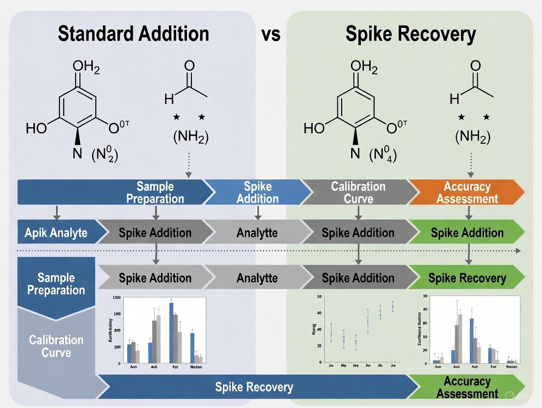
Standard Addition vs. Spike Recovery: A Strategic Guide to Accuracy Assessment in Analytical Science
This article provides a comprehensive comparison of two fundamental accuracy assessment methods in analytical chemistry: standard addition and spike recovery.
Standard Addition vs. Spike Recovery: A Strategic Guide to Accuracy Assessment in Analytical Science
Abstract
This article provides a comprehensive comparison of two fundamental accuracy assessment methods in analytical chemistry: standard addition and spike recovery. Tailored for researchers, scientists, and drug development professionals, it explores the core principles, appropriate applications, and procedural details for each technique. Readers will gain practical insights for selecting the correct method, troubleshooting common issues like matrix effects, and applying rigorous validation standards to ensure data reliability in complex matrices, from environmental samples to biopharmaceutical products.
Core Principles and Purpose: Demystifying Accuracy Assessment
Defining Accuracy, Precision, and the Challenge of Matrix Effects
In quantitative analysis, particularly within fields like forensic toxicology and environmental science, achieving reliable measurements is paramount. Two fundamental concepts, accuracy and precision, are used to describe the quality of these measurements, while matrix effects present a significant challenge to obtaining them. Accuracy refers to the closeness of a measurement to the true value, whereas precision describes the closeness of repeated measurements to each other [1]. This guide objectively compares two primary methodological approaches—standard addition and spike recovery (internal standard methods)—used to combat matrix effects and ensure accurate, precise results in complex samples.
Defining Core Concepts: Accuracy and Precision
Accuracy
Accuracy measures the overall correctness of a result. In classification tasks, it is defined as the proportion of all correct predictions (both positive and negative) among the total number of cases examined [2]. The formula is: Accuracy = (True Positives + True Negatives) / (True Positives + False Positives + True Negatives + False Negatives) [2] [3] [1]. However, accuracy alone can be misleading, especially when dealing with imbalanced datasets, where one class is significantly more frequent than another [2] [1].
Precision
Precision, also called positive predictive value, measures a model's reliability when it predicts the positive class. It answers the question: "Of all instances predicted as positive, how many are actually positive?" [2] [1]. It is calculated as: Precision = True Positives / (True Positives + False Positives) [2] [3]. A high precision indicates a low rate of false positives, which is crucial when the cost of a false alarm is high [1].
Recall
While not in the article's title, recall is a related and crucial metric for understanding the trade-offs with precision. Recall, or true positive rate, measures the ability to find all positive instances. It answers: "Of all actual positive instances, how many did we correctly identify?" [2] [1]. It is calculated as: Recall = True Positives / (True Positives + False Negatives) [2] [3]. A high recall indicates a low rate of false negatives.
Table 1: Summary of Key Performance Metrics
| Metric | Definition | Focus | When it Matters |
|---|---|---|---|
| Accuracy | Overall proportion of correct predictions | Overall correctness | Balanced datasets; when false positives and false negatives have similar costs [2]. |
| Precision | Proportion of correct positive predictions | Reliability of a positive prediction | False positives are costly (e.g., spam detection) [2] [1]. |
| Recall | Proportion of actual positives correctly identified | Finding all positive cases | False negatives are costly (e.g., disease screening, fraud detection) [2] [1]. |
The Fundamental Challenge: Matrix Effects
Matrix effects occur when the chemical composition of a sample (the "matrix") interferes with the measurement of the target analyte. This interference can alter the analytical signal, leading to either suppression or enhancement, and ultimately resulting in inaccurate quantification [4]. Matrix effects are a pervasive problem in the analysis of complex samples such as blood, soil, treated effluent, and food products [5] [4] [6].
The following diagram illustrates how matrix effects influence different calibration methods.
Diagram 1: The impact of matrix effects on different calibration methods. Standard addition and internal standards are designed to compensate for these effects.
Method Comparison: Standard Addition vs. Spike Recovery
To counteract matrix effects, scientists employ robust calibration techniques. The two most prominent are the standard addition method and methods involving spiked recovery, which include the use of internal standards.
Standard Addition Method
The standard addition method involves spiking the sample itself with known concentrations of the target analyte [4] [6]. Multiple aliquots of the sample are prepared with increasing spike levels, and the analytical response is measured for each. The key principle is that the added standard undergoes the exact same sample preparation and matrix influences as the native analyte, effectively correcting for both matrix effects and recovery losses [4]. The concentration of the original sample is determined by extrapolating the calibration line to the x-intercept [6].
Experimental Protocol for Standard Addition (as used in Forensic Toxicology) [6]:
- Sample Aliquoting: Aliquot a sample (e.g., blood) into four replicates.
- Spiking: Leave one replicate unspiked ("blank"). Fortify the remaining three replicates with known, increasing concentrations of the target drug standard.
- Sample Preparation: Process all aliquots (including the blank) through the entire analytical method (e.g., liquid-liquid extraction).
- Instrumental Analysis: Analyze all aliquots using the instrument (e.g., LC-MS/MS).
- Data Plotting & Calculation: Plot the peak area ratio (analyte/internal standard) against the spiked concentration. Perform linear regression. The absolute value of the x-intercept of the plotted line gives the concentration of the drug in the original sample. A correlation coefficient (R²) of >0.98 is typically required [6].
Spike Recovery and Internal Standard Method
Spike recovery is a procedure used to evaluate the accuracy of an analytical method by adding a known amount of analyte to a sample and measuring how much is recovered [7]. The internal standard method is a specific, powerful application of this principle. It involves adding a known amount of a foreign compound (the internal standard) to both calibration standards and samples before any processing [5] [4]. This internal standard should behave similarly to the analyte but be distinguishable by the instrument. By measuring the ratio of the analyte signal to the internal standard signal, the method can correct for losses during sample preparation and variations in instrument response [4].
Experimental Protocol for Internal Standard Method [4]:
- Internal Standard Addition: A consistent amount of a suitable internal standard is added to all calibration standards, quality control samples, and unknown samples at the very beginning of the analysis.
- Calibration Curve: A calibration curve is prepared using blank matrix spiked with known concentrations of the analyte and the internal standard.
- Sample Processing: All samples and standards are processed through the entire analytical method.
- Quantification: The analyte-to-internal standard response ratio is calculated for each sample. The concentration of the analyte in the unknown sample is determined by interpolating this ratio against the calibration curve.
Table 2: Objective Comparison of Standard Addition and Internal Standard Methods
| Feature | Standard Addition | Internal Standard Method |
|---|---|---|
| Principle | Spiking the sample itself with analyte [4] [6]. | Adding a different, known compound (internal standard) to all samples and standards [4]. |
| Primary Use | Ideal for single-analyte quantification in unique or variable matrices; often used when matched matrix blanks are unavailable [4] [6]. | Ideal for high-throughput, multi-analyte methods where sample losses are expected [4]. |
| Correction For | Matrix effects and recovery rate (as the standard undergoes the entire process with the analyte) [4]. | Losses during sample preparation and instrument variability [4]. May require matrix-matched standards for matrix effects. |
| Throughput | Low; labor-intensive, requires multiple preparations per sample [4]. | High; efficient for batch processing of many samples [4]. |
| Data Analysis | Extrapolation to x-intercept from a sample-specific curve [6]. | Interpolation from a single, shared calibration curve [4]. |
| Reported Experimental Data (Overall Accuracy) | Successfully implemented for NPS quantification in forensic casework with high correlation (R² > 0.98) [6]. | In a land cover map study, internal methods showed overall accuracy between 42% and 72% [8]. |
The Scientist's Toolkit: Essential Research Reagents and Materials
The following table details key materials and reagents essential for implementing the discussed quantitative methods.
Table 3: Essential Reagents and Materials for Quantitative Analysis
| Item | Function |
|---|---|
| High-Purity Analytical Standards | Used to prepare calibration spikes in both standard addition and internal standard methods. They serve as the reference for quantification [4] [6]. |
| Deuterated or Analog Internal Standards | A type of standard, ideally isotopically labeled (e.g., deuterated), that mimics the analyte's behavior to correct for sample preparation losses and instrument variation [4]. |
| Blank Matrix | The analyte-free sample material (e.g., drug-free blood, pure solvent) used to prepare calibration standards for the internal standard method and to verify the absence of interference [4]. |
| Quality Control (QC) Samples | Samples with known concentrations of the analyte, processed alongside unknowns to monitor the accuracy and precision of the analytical run over time [7]. |
| Extraction Solvents (e.g., N-butyl chloride) | Used in sample preparation to isolate the analyte from the complex sample matrix, improving detection and reducing interference [6]. |
The choice between standard addition and internal standard methods is not a matter of which is universally superior, but which is more appropriate for the specific analytical challenge. The following diagram summarizes the decision-making workflow.
Diagram 2: A workflow to guide the selection of an appropriate calibration method to ensure accuracy and precision.
For the analysis of unique or variable samples where matrix effects are severe, standard addition provides a robust, sample-specific solution, though at the cost of throughput [4] [6]. For routine, high-volume analysis, the internal standard method offers an efficient and reliable means of control, provided a suitable standard is available [4]. Ultimately, a deep understanding of accuracy, precision, and the sources of error in a measurement allows scientists to select the optimal strategy for validating their results.
What is Standard Addition? The Extrapolation Method for Complex Samples
In analytical chemistry, the accurate quantification of an analyte in a complex sample is often compromised by the matrix effect, where other components in the sample interfere with the analytical signal, leading to inaccurate results [9] [10]. The standard addition method is a calibration technique designed to overcome this challenge. Unlike external calibration, which uses separate standard solutions, standard addition involves adding known quantities of the analyte directly to the sample itself [11]. This ensures that the matrix composition is nearly identical for all measured solutions, allowing the analytical signal to be corrected for the interfering effects of the sample matrix [12] [10].
This guide focuses on the extrapolation method of standard addition, which is the most common and recommended approach for determining the original analyte concentration in a sample [13] [14]. We will objectively compare its performance and procedural details against the spike recovery method, another technique used for accuracy assessment in complex matrices.
The Principle and Workflow of the Extrapolation Method
The core principle of the standard addition extrapolation method is that by adding known amounts of standard to the sample, the matrix effect remains constant across all measurements. The unknown concentration is then determined by extrapolating the calibration line back to the point of zero signal [13] [15].
Theoretical Foundation
In an ideal system free of measurement error, the relationship between the analytical signal (Y) and the analyte concentration (C) is linear and follows the equation: [ Y = \beta C ] When an unknown sample with an initial concentration ( C0 ) is spiked with a standard addition of concentration ( x ), the observed signal becomes: [ Y(C0 + x) = \beta (C0 + x) = \beta C0 + \beta x ] This equation, ( Y = \beta0 + \beta1 x ), defines the standard addition curve, where the slope (( \beta1 )) represents the sensitivity of the method, and the y-intercept (( \beta0 )) is the signal due to the original analyte in the sample. The unknown concentration ( C0 ) is calculated from the ratio of the intercept to the slope: ( C0 = \beta0 / \beta1 ), which corresponds to the negative x-intercept [14].
Graphical Interpretation and Calculation
In practice, the x-intercept is found graphically or via linear regression [13] [15]. The absolute value of this intercept gives the concentration of the analyte in the original sample. The following diagram illustrates this workflow and the underlying mathematical relationships.
Experimental Protocol for the Extrapolation Method
The successful application of the standard addition extrapolation method requires a meticulous experimental setup to ensure the matrix effect is constant across all measurements [11] [9].
Step-by-Step Procedure
- Preparation of Test Solutions: Obtain several identical aliquots (e.g., 5-6) of the sample. Each aliquot should contain the same volume of the unknown sample, ( V_x ) [11] [9].
- Standard Spiking: To all but one of the aliquots, add progressively increasing, but known, volumes (( Vs )) of a standard solution with a known, high concentration (( Cs )). One aliquot is left unspiked (this is the "0" addition point) [13] [9].
- Dilution to Constant Volume: Dilute each aliquot—both spiked and unspiked—to the same final volume using an appropriate solvent. This crucial step ensures that the sample matrix is identical in all solutions, differing only in the total analyte concentration [11].
- Measurement of Instrument Response: Analyze each prepared solution using the chosen instrumental technique (e.g., AAS, ICP-MS, spectroscopy) and record the analytical signal (S) for each [9].
- Data Analysis and Extrapolation:
- Plot the measured signal (y-axis) against the concentration of the added standard in the final solution (x-axis). The added concentration is calculated from ( Vs ) and ( Cs ), accounting for the final dilution [13].
- Perform a linear regression analysis on the data points to obtain the equation of the line: ( Y = mX + b ), where ( m ) is the slope and ( b ) is the y-intercept.
- Calculate the x-intercept by setting ( Y=0 ) and solving for ( X ): ( X{intercept} = -b/m ). The original concentration of the analyte in the sample, ( Cx ), is the absolute value of this intercept [15].
Key Research Reagent Solutions
The following table details essential materials and reagents required for a typical standard addition experiment.
| Reagent/Material | Function in the Experiment | Specification Notes |
|---|---|---|
| Primary Analyte Standard | Provides the known quantity of analyte for spiking; the reference for quantification. | High-purity certified reference material (CRM) to ensure accuracy [11]. |
| Sample Matrix | Contains the unknown concentration of the analyte (( C_x )) to be determined. | Should be homogeneous; volume per aliquot (( V_x )) must be consistent [9]. |
| Dilution Solvent | Brings all sample aliquots to an identical final volume. | Must be high-purity and compatible with both the sample matrix and the instrument [11]. |
| Instrument Calibrants | For initial instrument calibration and verification of linear response. | May be prepared in a simple matrix (e.g., acidic water) to establish initial sensitivity [16]. |
Quantitative Comparison: Standard Addition vs. Spike Recovery
While both standard addition and spike recovery are used to assess method accuracy in complex matrices, their applications, calculations, and performance differ significantly. The table below summarizes a quantitative and procedural comparison based on experimental data and statistical evaluations.
| Comparison Parameter | Standard Addition (Extrapolation) | Spike Recovery | ||
|---|---|---|---|---|
| Primary Objective | Direct determination of unknown analyte concentration (( C_x )) in a complex sample [9]. | Assessment of the accuracy and bias of an existing analytical method [17]. | ||
| Core Principle | Extrapolation of a linear calibration curve to the x-axis to find ( C_x ) [13] [15]. | Calculation of the percentage recovery of a known amount of analyte added to the sample [17]. | ||
| Typical Procedure | Multiple additions (e.g., 5-6 points) of standard to the sample to construct a linear curve [11]. | Typically a single-level or two-level addition of analyte to the sample. | ||
| Key Mathematical Formula | ( C_x = \left | \frac{-b}{m} \right | ) from ( Y = mX + b ) [15]. | ( \% \text{Recovery} = \frac{C{\text{spiked}} - C{\text{unspiked}}}{\text{Added Concentration}} \times 100 ) |
| Handling of Matrix Effects | Excellent compensation for rotational matrix effects (those affecting slope) [14]. | Can indicate the presence of a matrix effect but does not inherently correct for it in the final reported ( C_x ). | ||
| Statistical Performance (Trueness & Precision) | Considered most recommendable with respect to low bias and variability when underlying assumptions are met [14]. | Useful for bias assessment, but a single-point recovery does not provide the same statistical confidence as a multi-point standard addition. | ||
| Estimated Uncertainty | Can be approximated using error propagation on regression parameters [11] [14]. | Generally reported as the standard deviation of replicate recovery measurements. | ||
| Sample Consumption | Higher, due to the need for multiple aliquots [11]. | Lower, as it can be performed with fewer aliquots. | ||
| Best Application Context | Quantification in samples with unknown or variable matrix that causes rotational effects [12] [10]. | Validation of an established method for a known matrix, or routine quality control to check for bias [17]. |
The standard addition extrapolation method is a powerful tool for achieving accurate quantification in complex samples where matrix effects pose a significant challenge to conventional calibration. Its principal strength lies in its ability to compensate for rotational matrix effects by maintaining a consistent matrix background across all calibration points, thereby producing a more reliable estimate of the true unknown concentration [14].
For researchers and drug development professionals, the choice between standard addition and spike recovery hinges on the specific analytical objective. Standard addition is the method of choice for definitive concentration determination in unknown or highly variable matrices, such as in the analysis of active pharmaceutical ingredients in biological fluids or contaminants in environmental samples [9]. In contrast, spike recovery is a vital quality assurance tool best suited for validating the accuracy of an existing method and monitoring for systematic bias during routine analysis [17]. Understanding the operational protocols, statistical foundations, and comparative performance of these two methods allows scientists to make an informed decision that ensures data integrity and supports robust analytical outcomes.
What is Spike Recovery? The Percent Recovery Validation Technique
Spike recovery, also known as percent recovery, represents a fundamental validation technique used across analytical chemistry and bioanalysis to assess method accuracy by measuring how effectively an analytical procedure can detect a known quantity of analyte added to a sample matrix. This technique is particularly valuable for identifying matrix effects—where components within a sample interfere with analyte detection—and for validating that an assay provides accurate quantitative results despite potential interferents. As one approach within a broader framework of accuracy assessment methods, spike recovery serves a distinct purpose compared to alternative techniques like the standard addition method, each with specific advantages, limitations, and optimal application contexts. This guide provides researchers and drug development professionals with a comprehensive comparison of these methodologies, supported by experimental data and implementation protocols.
Understanding Spike Recovery and Its Purpose
Spike recovery experiments involve introducing ("spiking") known amounts of a target analyte into specific sample matrices and measuring the percentage of this added material that is recovered through the analytical method [18] [19]. The core purpose is to evaluate whether the sample matrix affects the accuracy of analyte detection and quantification, which is crucial for validating analytical methods used in pharmaceutical development, clinical diagnostics, and environmental testing [18] [20].
The fundamental principle underlying spike recovery assessment is the comparison between analyte behavior in a controlled diluent versus within a complex sample matrix [18]. When an analyte is introduced into a biological matrix such as serum, urine, or tissue homogenate, components within that matrix may enhance or suppress detection signals, leading to inaccurate quantification [19] [21]. These matrix effects can result from various factors including high or low pH, elevated protein or salt concentrations, or the presence of detergents or organic solvents [19]. In medicinal herb analysis, for instance, spike recovery helps evaluate whether extraction methods effectively liberate native analytes that may be enwrapped within herbal materials, though its reliability in this context requires careful validation of extraction efficiency [20].
Spike recovery testing is particularly valuable during method development and validation, as it helps researchers identify optimal sample preparation procedures, establish appropriate dilution factors, and verify that matrix effects do not compromise analytical accuracy [18] [19]. For drug development professionals, this technique provides critical assurance that analytical methods will perform reliably when applied to complex biological samples throughout the drug development pipeline—from in-process monitoring to final product quality control [19].
Experimental Protocols for Spike Recovery Assessment
Standard Spike Recovery Protocol
The standard spike recovery protocol follows a systematic approach to evaluate matrix effects:
Sample Preparation: Begin with aliquots of the sample matrix. For each sample type being evaluated, prepare multiple aliquots to test different spike concentrations [19].
Spiking Procedure: Add known amounts of the purified analyte standard to the sample matrix. Typically, 3-4 concentration levels covering the analytical range of the assay are used, with the lowest spiked concentration being at least 2 times the Limit of Quantitation (LOQ) of the assay [19]. The volume of spike solution should be small relative to the sample volume (generally not exceeding 10% of total volume) to minimize dilution of the sample matrix [22].
Control Preparation: In parallel, prepare identical spikes in the standard diluent used for assay calibration curves. Additionally, prepare a control sample where the matrix is diluted with zero standard or plain diluent to determine the endogenous contribution of the analyte prior to spiking [19].
Analysis: Analyze all samples using the established analytical method (e.g., ELISA, LC-MS, spectrophotometry) [18] [21].
Calculation: Calculate percent recovery using the formula:
Recovery % = [(Total measured concentration - Endogenous concentration) / Spiked concentration] × 100
Where:
The following diagram illustrates the experimental workflow for spike recovery assessment:
Acceptance Criteria and Interpretation
According to industry standards, recovery values within 75% to 125% of the spiked concentration are generally considered acceptable for most analytical applications, though specific validation guidelines may define different ranges based on application requirements [19]. The International Council for Harmonisation (ICH), FDA, and EMA guidelines on analytical procedure validation typically endorse these ranges for bioanalytical method validation [19].
When interpreting spike recovery results:
- Recovery ≈ 100%: Indicates minimal matrix interference and validates the analytical method for that specific sample matrix [18].
- Recovery < 75% (Under-recovery): Suggests matrix components are suppressing analyte detection, potentially due to binding, degradation, or interference with detection mechanisms [19].
- Recovery > 125% (Over-recovery): Indicates matrix components are enhancing detection, possibly through non-specific binding or interference with assay components [19].
Comparative Analysis: Spike Recovery vs. Standard Addition Method
While spike recovery and standard addition both involve adding known quantities of analyte to samples, they represent fundamentally different approaches to accuracy assessment. The following table compares their key characteristics:
| Characteristic | Spike Recovery Method | Standard Addition Method (SAM) |
|---|---|---|
| Primary Purpose | Validate method accuracy in specific matrices [18] [19] | Quantify analytes in complex matrices without blank references [23] |
| Experimental Design | Compare recovery between sample matrix and standard diluent [18] | Multiple additions of standard to the same sample with extrapolation [23] |
| Matrix Requirements | Requires compatible blank or reference matrix [18] | No blank matrix required [23] |
| Data Interpretation | Percent recovery calculated against expected value [19] | Concentration determined by extrapolating calibration curve to x-axis [23] |
| Best Applications | Method validation, quality control, matrix effect screening [18] [19] | Analyzing samples with unknown matrix effects; endogenous analytes [21] [23] |
| Throughput | Higher throughput for multiple samples [18] | Lower throughput; labor-intensive [23] |
| Limitations | Limited value without appropriate blank matrix [20] | Time-consuming; not practical for large sample batches [23] |
The standard addition method follows a distinct experimental approach, particularly valuable when analyzing samples where a blank matrix is unavailable or when matrix effects are significant and variable between samples [23]. The method involves spiking the same sample with increasing known amounts of analyte and extrapolating back to determine the original concentration [23].
The following decision pathway helps researchers select the appropriate accuracy assessment method:
Experimental Data and Case Studies
Representative Spike Recovery Data
Spike recovery experiments generate quantitative data that demonstrate method performance across different matrices and conditions. The following table compiles representative recovery data from published studies:
| Sample Matrix | Analyte | Spike Level | Recovery % | Reference Method |
|---|---|---|---|---|
| Human Urine [18] | IL-1 beta | 15 pg/mL (Low) | 86.3% ± 9.9% | ELISA |
| Human Urine [18] | IL-1 beta | 40 pg/mL (Medium) | 85.8% ± 6.7% | ELISA |
| Human Urine [18] | IL-1 beta | 80 pg/mL (High) | 84.6% ± 3.5% | ELISA |
| Chinese Liquor [24] | Cyanide | Trace levels | 91.5-98.5% | Automated Distillation-Flow Analysis |
| Final Drug Product [19] | HCP | 20 ng/mL | 95% | ELISA |
| Rhei Rhizoma [20] | Aloe-emodin | Herbal analysis | 22.8-93.3%* | HPLC |
*Variable recovery depending on extraction efficiency [20]
Troubleshooting Poor Spike Recovery
When spike recovery falls outside acceptable ranges, several corrective strategies can be implemented:
- Modify Standard Diluent: Alter the standard diluent composition to more closely match the sample matrix. For culture supernatant samples, for instance, using culture medium as the standard diluent may improve recovery [18].
- Optimize Sample Dilution: If neat biological samples show poor recovery, test the samples upon dilution in standard diluent. A 1:1 dilution of serum in standard diluent often corrects recovery issues, provided the analyte remains detectable [18].
- Adjust Matrix Composition: Modify the sample matrix pH to match the optimized standard diluent or add carrier proteins like BSA to stabilize the analyte [18].
- Enhance Sample Preparation: For complex matrices like medicinal herbs, optimize extraction procedures to ensure native analytes are efficiently extracted [20].
Essential Research Reagents and Materials
Successful spike recovery experiments require specific reagents and materials carefully selected for each application:
| Reagent/Material | Function | Application Notes |
|---|---|---|
| Purified Analyte Standard | Spike material of known concentration | Should be identical to native analyte; high purity essential [18] |
| Matrix-Matched Diluent | Standard diluent resembling sample matrix | Improves recovery when sample matrix affects detection [18] |
| Appropriate Negative Controls | Measure endogenous analyte levels | Includes zero standard samples without spike [19] |
| Quality Antibody Pairs | Detection and capture antibodies for immunoassays | Critical for ELISA-based recovery assays [18] [25] |
| Stable Isotope-Labeled Internal Standards | Correction for matrix effects in MS | Ideal but expensive; corrects for ionization suppression/enhancement [21] |
| Sample Preparation Materials | Extraction solvents, filters, solid-phase columns | Optimization crucial for complete analyte extraction [20] |
Advanced Applications and Method Validation
Dilutional Linearity and Parallelism Testing
Spike recovery represents one component of a comprehensive method validation strategy that should also include:
- Dilutional Linearity: Assesses whether sample dilution produces proportional concentration changes. This experiment involves spiking a known amount of analyte into a sample above the assay's upper detection limit, then serially diluting it below the lower limit of quantification [18] [25]. Good linearity indicates minimal matrix effects across the assay range.
- Parallelism Testing: Evaluates whether antibody binding affinity differs between the endogenous analyte and the standard curve analyte. Natural samples with high analyte concentrations are serially diluted and analyzed; a high coefficient of variation (%CV) between dilutions indicates potential matrix effects on antibody binding [25].
Limitations and Critical Considerations
While spike recovery is a valuable validation technique, researchers should recognize its limitations:
- Extraction Efficiency Concerns: For solid samples like medicinal herbs, spiked analytes may be more easily extracted than native analytes enclosed within cellular structures, potentially leading to misleading recovery values [20].
- Matrix Variability: Recovery may vary between individual sample sources (e.g., different donor sera), necessitating assessment across multiple lots [18].
- Concentration Dependence: Recovery rates may differ at various analyte concentrations, requiring evaluation across the assay range [18] [19].
- Non-Specific Interference: Components in complex matrices may cause non-specific binding or signal interference not detected in standard spike recovery experiments [19] [21].
Spike recovery assessment serves as an indispensable technique in the analytical scientist's toolkit, providing critical validation of method accuracy across diverse sample matrices. While particularly valuable for quality control in regulated environments like drug development, it functions most effectively as part of a comprehensive validation strategy that may include alternative approaches like standard addition for particularly challenging matrices. By implementing robust spike recovery protocols, troubleshooting poor recovery systematically, and interpreting results within established acceptance criteria, researchers can generate reliable, accurate data supporting drug development, clinical diagnostics, and environmental monitoring. As analytical challenges grow with increasingly complex samples and lower detection limits, the principles of spike recovery remain foundational to demonstrating method validity and data integrity.
Historical Context and Evolution of the Two Methods
In the field of analytical chemistry, ensuring the accuracy of quantitative measurements is paramount, particularly when analyzing complex sample matrices. Two principal methods, Standard Addition and Spike Recovery, have been developed to assess and correct for matrix effects that can interfere with analyte detection [18]. The standard addition method involves adding known amounts of analyte directly to the sample of interest, allowing for quantification by extrapolation [11]. Spike recovery, often used in method validation, assesses accuracy by comparing the measured concentration of a known spike to its true value [18]. This guide provides an objective comparison of these methods, tracing their historical development, detailing their experimental protocols, and evaluating their performance through structured data and visual workflows. Designed for researchers, scientists, and drug development professionals, this analysis situates the methods within a broader thesis on accuracy assessment, highlighting their respective strengths, limitations, and ideal applications.
Historical Development and Evolution
The two methods have distinct origins and evolutionary paths, reflecting their different roles in analytical science.
Table 1: Historical Context of Standard Addition and Spike Recovery
| Aspect | Standard Addition Method | Spike Recovery Assessment |
|---|---|---|
| Origin Date & Context | First reported in 1937 by Hans Hohn for polarographic analysis of zinc [11] [26]. | Emerged as a fundamental practice for method validation in analytical chemistry and immunoassays [18]. |
| Key Initial Purpose | To determine analyte concentration in complex samples with matrix effects without needing a blank matrix [11]. | To validate the accuracy of an analytical method by determining if the sample matrix affects analyte detection [18]. |
| Evolution of Application | Expanded from polarography to spectroscopy (1950s), X-ray fluorescence (1954), and natural complex mediums like seawater (1955) [26]. Now used in advanced fields like forensic toxicology for Novel Psychoactive Substances (NPS) and immunoassays with non-linear curves [26] [6]. | Widely adopted as a standard step in method validation across various techniques, including ELISA and chromatography, to ensure reliability [18]. |
| Technological Drivers | Adaptation to various instrumental techniques (AAS, HPLC, MS) and complex samples. Recent focus on adapting the method for non-linear immunoassay calibration curves [26] [6]. | The need for robust quality control in the analysis of complex biological and environmental samples, driving standardized validation protocols [18]. |
The standard addition method was revolutionary because it addressed a fundamental problem in analyzing real-world samples: the matrix effect. By using the sample itself as the primary matrix for the calibration, it inherently corrected for both preparation losses and instrumental matrix effects [27]. Its recent evolution involves sophisticated computational approaches to extend its use to non-linear calibration models, such as those in immunoassays [26].
Spike recovery, while also dealing with matrix effects, evolved more as a quality control tool to verify that a pre-established analytical method, often using an external calibration curve, performs accurately for a specific sample type [18]. Its history is less about a single inventor and more about the systematic development of analytical quality assurance.
Figure 1: The parallel evolutionary pathways of Standard Addition (blue) and Spike Recovery (yellow).
Methodological Principles and Workflows
The core distinction lies in how the two methods use the spiked analyte to calculate accuracy and correct for the sample matrix.
Standard Addition Method
This method is used for direct quantification of the unknown. It involves preparing multiple aliquots of the sample, spiking them with increasing known amounts of the analyte, and then extrapolating back to find the original concentration [27] [11].
Key Protocol Steps [11] [9] [6]:
- Sample Aliquoting: Divide the sample with unknown concentration ( C_x ) into several equal aliquots.
- Spiking: Add known and varying concentrations of a standard solution (e.g., 0, 1, 2, 3, 4, 5 mL of a standard with concentration ( C_s )) to these aliquots. One aliquot remains unspiked.
- Dilution: Dilute all aliquots to the same final volume.
- Analysis: Measure the instrumental response (e.g., peak area, absorbance) for each solution.
- Data Plotting & Calculation: Plot the instrumental response (y-axis) against the concentration of the added standard (x-axis). Perform linear regression. The absolute value of the x-intercept (where y=0) corresponds to the original analyte concentration ( C_x ) in the sample.
Figure 2: Standard Addition experimental workflow for quantification.
Spike Recovery Assessment
This method is used to validate the accuracy of an existing analytical procedure. A known amount of analyte is added to the sample, and the measured concentration is compared to the expected value [18].
Key Protocol Steps [18]:
- Sample Preparation: Obtain the test sample matrix.
- Spiking: Add a known concentration of analyte ("spike") to one or more aliquots of the sample. A separate, unspiked sample is also analyzed to determine the endogenous level.
- Analysis: Analyze both the spiked and unspiked samples using the validated method (which typically uses an external calibration curve).
- Calculation: The recovery is calculated as: ( \text{Recovery} \% = \frac{\text{(Measured concentration in spiked sample)} - \text{(Measured concentration in unspiked sample)}}{\text{Theoretical spike concentration}} \times 100\% ) A recovery close to 100% indicates minimal matrix interference.
Figure 3: Spike Recovery workflow for method validation.
Comparative Experimental Data and Performance
The following tables summarize experimental data and key performance metrics for both methods, highlighting their operational characteristics and typical outcomes.
Table 2: Summary of Experimental Data and Performance Metrics
| Parameter | Standard Addition | Spike Recovery |
|---|---|---|
| Primary Objective | Direct quantification of unknown [11] | Validation of method accuracy [18] |
| Calibration Model | Internal (in the sample matrix) [6] | External (in a clean solvent or blank matrix) [27] |
| Key Quantitative Output | Original analyte concentration ( C_x ) [9] | Percentage Recovery (%) [18] |
| Typical Recovery Range | Argued to be effectively 100% as it accounts for losses and matrix effects [27] | Ideal range 95-105%; acceptable range can be 80-120% depending on the method [18] |
| Data from Literature | Successfully quantified NPS (e.g., isotonitazene) in forensic casework with R² > 0.98 [6]. Quantified testosterone in milk/serum with recoveries of 70-118% [26]. | Example: ELISA for IL-1 beta in human urine showed mean recoveries of 84.6-86.3% across low/medium/high spikes [18]. |
| Handles High Background | Limited; high native concentration flattens curve slope, causing significant deviations [27]. | Can be challenging if unspiked level is high and impacts the calibration curve dynamic range. |
| Sample Consumption | Higher; requires multiple aliquots per sample [28] | Lower; can often be performed with fewer aliquots [18] |
Table 3: Operational Comparison and Practical Considerations
| Aspect | Standard Addition | Spike Recovery |
|---|---|---|
| Throughput | Lower; requires constructing a curve for each sample [27] [28] | Higher; a single calibration curve can be used for many samples [27] |
| Labor & Cost | Higher (more labor-intensive, consumes more sample and reagents) [27] [28] | Lower [27] |
| Matrix Effect Correction | Excellent; corrects for both proportional and translational effects on recovery and signal [27] [11] | Good for identifying effects; requires separate optimization (e.g., diluent alteration) to correct them [18] |
| Need for Blank Matrix | Not required [28] | Required for preparing calibration standards in traditional external calibration [28] |
| Ideal Application Context | Unique or complex samples where a blank matrix is unavailable; low-volume testing of specific analytes (e.g., NPS in forensics) [28] [6] | High-throughput routine analysis; batch processing of similar samples; method development and validation [27] [18] |
Essential Research Reagent Solutions
Successful implementation of both methods relies on a core set of materials and reagents.
Table 4: Key Reagents and Materials for Experimental Implementation
| Reagent / Material | Function and Importance | Application in Methods |
|---|---|---|
| High-Purity Analyte Standard | Serves as the reference for spiking. Purity is critical for accurate concentration calculations. | Both |
| Appropriate Internal Standard (IS) | Corrects for variability in sample preparation and instrument response. Often isotopically labeled for MS. | Common in Standard Addition for LC-MS/MS [6]; used in calibrated methods for Spike Recovery. |
| Matrix-Matched Solvents & Buffers | (For Spike Recovery) Used to prepare the external calibration curve to mimic the sample matrix and reduce bias [18]. | Primarily Spike Recovery |
| Sample Diluent (Optimized) | Used to dilute samples to within the analytical range. Composition can be optimized to improve recovery by matching pH or adding protein [18]. | Primarily Spike Recovery |
| Sample Collection Vessels & Pipettes | Ensure accurate and precise liquid handling. Critical for the multiple volume additions in Standard Addition [9]. | Both |
| Solid-Phase Extraction (SPE) / Liquid-Liquid Extraction (LLE) Materials | For sample clean-up and pre-concentration. Can reduce matrix interference and improve signal [6]. | Both |
For researchers and scientists engaged in drug development and analytical testing, selecting the appropriate accuracy assessment method is fundamental to generating reliable data. Two principal techniques—standard addition and spike recovery—are employed to validate analytical methods, particularly when dealing with complex sample matrices that can interfere with measurements. While both methods involve adding a known quantity of analyte (a "spike") to a sample, their underlying principles, applications, and justifications differ significantly. This guide provides an objective comparison of these methods, supported by experimental data and protocols, to inform their justified use within a quality assurance framework.
Core Principles and Methodologies
Understanding Spike Recovery
Spike recovery is a quality assessment tool used to test whether an analytical method can accurately measure an analyte in a specific sample matrix. It evaluates the method's ability to recover a known quantity of analyte added to the sample, thereby detecting matrix interference that may cause under-recovery or over-recovery [29].
Experimental Protocol for Spike Recovery [29]:
- Determine Minimum Required Dilution (MRD): First, perform dilution linearity studies to establish the sample dilution at which antibody excess conditions are met and the working concentration is in an acceptable range.
- Prepare Spiked Samples: For each sample matrix type, spike 3-4 concentration levels covering the analytical range into the sample at the MRD. The lowest spiked concentration should be at least 2 times the assay's Limit of Quantitation (LOQ).
- Prepare Control: In parallel, prepare a control by diluting the sample with a "zero standard" (assay diluent) to determine the contribution of any endogenous analyte.
- Analysis and Calculation: Analyze all samples and calculate the percentage recovery using the formula:
- % Recovery = (Total HCP Measured in Spiked Sample - HCP in Negative Sample) / Spike Concentration × 100
- Acceptance Criteria: According to ICH, FDA, and EMA guidelines, recovery values within 75% to 125% are generally considered acceptable [29].
Understanding Standard Addition
The standard addition method is a quantitative analysis technique used to determine the concentration of an analyte in an unknown sample while directly compensating for matrix effects. Instead of using a separate calibration curve, it builds the calibration curve within the sample itself by measuring the response to incremental spikes [30] [9] [31].
Experimental Protocol for Standard Addition [9] [6]:
- Prepare Test Solutions: Aliquot a series of equal-volume portions of the sample with unknown concentration, Cx. To all but one of these aliquots, add increasing volumes, Vs, of a standard solution with a known concentration, Cs. One aliquot remains unspiked as the "blank".
- Measure Instrument Response: Analyze all solutions and measure the sensor response (e.g., peak area, spectroscopic intensity) for each.
- Plot and Calculate: Plot the measured response versus the spiked standard concentration (or volume). Perform linear regression to obtain a line with slope m and y-intercept b.
- Determine Unknown Concentration: The unknown original concentration, Cx, is calculated using the x-intercept of the line. The fundamental calculation is:
- Cx = -b/m (correcting for any dilution factors, often involving Cs and Vx) [9].
The workflow below illustrates the procedural steps and logical relationship for the Standard Addition Method.
Direct Comparison: Standard Addition vs. Spike Recovery
The table below summarizes the key characteristics, justifications, and limitations of each method to guide selection.
| Feature | Standard Addition | Spike Recovery |
|---|---|---|
| Primary Objective | Quantitative determination of unknown analyte concentration while correcting for matrix effects [30] [9]. | Validation of analytical method accuracy and detection of matrix interference in a specific sample type [29]. |
| Justified Use Cases | - Unknown or complex sample matrices (e.g., blood, soil, wastewater) [9] [31].- Analysis of emerging contaminants (e.g., novel psychoactive substances) where matched calibration standards are unavailable [6].- High-accuracy quantification of monoisotopic elements by ICP-MS [32]. | - Routine quality assessment during analysis of known sample types [17] [7].- Method validation and verification as per regulatory guidelines (ICH/FDA/EMA) [29].- Testing for interference in final drug product or in-process samples [29]. |
| Key Advantage | Corrects for both matrix effects and recovery rate losses; considered highly accurate as the added standard undergoes the same preparation as the sample [30]. | Simpler and more efficient for batch processing; provides direct measure of method accuracy under specific conditions [30] [29]. |
| Key Limitation | Labor-intensive, time-consuming, requires more sample and reagent, and not practical for high-throughput labs [30] [33]. | Does not inherently correct the reported sample concentration for matrix effects; only indicates the presence of interference [29]. |
| Data Output | A calculated value for the original analyte concentration in the sample [9]. | A percentage value indicating how much of the spiked analyte was measured [29]. |
| Acceptance Criteria | Based on the correlation coefficient (e.g., R² > 0.98) and quality of the linear fit [6]. | Typically 75%-125% recovery, though can be narrower (e.g., 80%-120% for metals) [29] [7]. |
Experimental Data and Supporting Evidence
Data from Spike Recovery Analysis
The following table exemplifies data generated from a spike and recovery experiment for a Host Cell Protein (HCP) ELISA assay, a common scenario in biopharmaceutical development [29].
| Sample Description | Spike Concentration (ng/mL) | Total HCP Measured (ng/mL) | % Spike Recovery |
|---|---|---|---|
| Final Product + Zero Standard | 0 | 6 | N/A |
| Final Product + 100 ng/mL Standard | 20 | 25 | 95% |
Calculation: (25 ng/mL - 6 ng/mL) / 20 ng/mL × 100 = 95% [29]. This value falls within the acceptable range of 75-125%, indicating minimal matrix interference for this sample under the tested conditions.
Application of Standard Addition in Forensic Toxicology
A compelling justification for standard addition is its use in quantifying emerging novel psychoactive substances (NPS) in forensic casework. One laboratory successfully implemented standard addition for drugs like isotonitazene (opioid) and eutylone (stimulant). Their protocol involved:
- Procedure: Analyzing four sample replicates: one unspiked and three spiked at different concentrations. The analyte-to-internal standard peak area ratio was plotted against the spike concentration [6].
- Calculation: The original drug concentration was determined by calculating the x-intercept of the plotted line, which required a correlation coefficient (R²) greater than 0.98 [6].
- Outcome: This approach provided a scientifically valid quantitative result where traditional external calibration methods were not yet established or validated [6].
The Scientist's Toolkit: Essential Research Reagents and Materials
Successful implementation of these methods requires specific, high-quality materials. The following table details key reagents and their functions.
| Item | Function in Experiment |
|---|---|
| Certified Reference Material (CRM) [31] | Provides a spike solution with a known and traceable analyte concentration, forming the basis for accurate additions in both methods. |
| Analyte-Free Matrix | Serves as the ideal blank and dilution solvent in spike recovery studies to capture variability from the sample preparation process [33]. |
| Internal Standard (IS) | Used in some standard addition variants (especially in mass spectrometry) to correct for instrument drift and preparation inconsistencies [6]. |
| Matrix-Matched Standards | For traditional calibration, these are used to contrast with standard addition; prepared by spiking the analyte into a blank matrix [30]. |
The choice between standard addition and spike recovery is not a matter of which is superior, but which is more justified for the specific analytical objective.
- Standard Addition is justified as the primary quantitative method when the sample matrix is complex, unpredictable, and introduces significant interference that cannot be easily mimicked for a traditional calibration curve. It is the method of choice for high-accuracy determination in unknown matrices, rare analytes, and novel drug substances [30] [6] [32].
- Spike Recovery is justified as a quality control and validation tool for monitoring the performance of an existing, validated method across different sample batches and matrices. It is essential for demonstrating the absence of matrix interference in regulated environments and for high-throughput laboratories where standard addition would be prohibitively slow [29] [7].
In practice, a robust quality assurance program may leverage both methods: spike recovery for ongoing validation of routine analyses, and standard addition to solve specific analytical challenges or to develop methods for new analytes in complex biological matrices.
Protocols in Practice: Implementing Standard Addition and Spike Recovery
This guide details the successive standard additions method, an analytical technique crucial for quantifying analyte concentration in complex sample matrices where interfering substances may skew results. The method involves adding known quantities of analyte directly to the sample to construct a matrix-matched calibration, effectively compensating for matrix effects that impair accuracy in traditional external calibration curves. We provide a comprehensive protocol, visual workflow, and comparative analysis against the spike recovery method, equipping researchers and drug development professionals with the knowledge to implement this technique for reliable analytical outcomes.
The successive standard additions method is a fundamental analytical technique used to determine the concentration of an analyte in a complex sample when the sample's matrix—the collection of all other components in the sample—causes a measurable interference known as a matrix effect [11] [9]. In such cases, using an external calibration curve prepared in a pure solvent can lead to significant inaccuracies, as the analyte in the pure standard may behave differently (e.g., produce a different instrument response) than the identical analyte embedded in the sample matrix [34]. The core principle of standard additions circumvents this issue by performing the calibration directly in the sample, thereby ensuring that the matrix is nearly identical for all measured solutions [11].
The underlying mathematics relies on the linear relationship between instrumental signal and analyte concentration. The signal (S) for the original sample is given by S = kC₀, where k is the sensitivity (the slope of the calibration line) and C₀ is the unknown analyte concentration. When a known volume of standard with concentration Cₛ is added, the signal becomes S = k(C₀ + Cₛ). By adding varying, known amounts of the analyte and measuring the corresponding signals, one can plot a curve. Extrapolating this line back to where the signal is zero reveals the negative value on the concentration axis corresponding to -C₀, allowing for the calculation of the original unknown concentration [11] [35]. This method is particularly valuable in applications like pharmaceutical testing (e.g., drug concentration in blood plasma), environmental monitoring (e.g., heavy metals in water), and food safety analysis [9].
Theoretical Foundation and Workflow
The successive standard additions method is predicated on the principle of extrapolation to account for matrix-induced changes in analytical sensitivity. Unlike external calibration, which assumes a consistent sensitivity (slope, k) between standards and samples, standard additions acknowledges that the matrix can alter k. By building the calibration curve within the sample itself, it inherently corrects for this "rotational" matrix effect, where the matrix changes the slope but not the intercept of the calibration function [14]. The method's validity rests on two key assumptions: a linear relationship between analyte concentration and measurement signal, and a blank signal not significantly different from zero [14].
The following diagram illustrates the logical sequence of the standard additions process, from sample preparation to the final calculation of the unknown concentration.
The logical workflow culminates in a graphical representation of the data. A plot of instrument signal versus spiked analyte amount (or concentration) produces a straight line. The x-intercept of this line, found by setting the signal (S) to zero in the regression equation S = m*x + b, yields the value of -C₀. The absolute value of this intercept is the original concentration of the analyte in the unknown sample [11] [35]. This extrapolation is a critical differentiator from the spike recovery method, which typically relies on interpolation.
Experimental Protocol for Successive Standard Additions
Materials and Reagents
The following table lists the essential materials required to perform a successive standard additions experiment effectively.
| Item | Function & Specification |
|---|---|
| Analytical Sample | The solution containing the analyte of interest at an unknown concentration (C₀). Matrix should be representative. |
| Standard Solution | A solution with a precisely known, high concentration of the analyte (Cₛ). Purity should be certified. |
| Diluent/Solvent | A solvent matching that used for the standard solution and for diluting samples to volume (e.g., purified water, acid, buffer). |
| Volumetric Glassware | Precision pipettes, volumetric flasks, or cylinders for accurate transfer and dilution of samples and standards. |
| Analytical Instrument | The measurement system (e.g., AAS, ICP-MS, HPLC, UV-Vis) with validated performance for the analyte. |
Step-by-Step Procedure
This protocol outlines the successive standard additions method for determining an unknown analyte concentration in a complex matrix.
- Prepare Test Solutions: Obtain several identical aliquots (e.g., 10 mL each) of the sample (Vₓ) with unknown concentration (Cₓ). The number of aliquots determines the number of data points; a minimum of three additions plus the unspiked sample is recommended for a reliable regression line [11] [9].
- Spike the Aliquots: To all but one of the aliquots, add increasing, known volumes (Vₛ) of a standard solution with a known, high concentration (Cₛ). For example, add 0, 1, 2, 3, and 4 mL of the standard. The one aliquot receiving no standard serves as the "0" addition point [11].
- Dilute to Volume: Dilute each solution (including the unspiked sample) to the same final volume (e.g., 25 mL) using an appropriate diluent. This crucial step ensures that the matrix is nearly identical across all solutions and that the only variable is the total amount of analyte [11] [9].
- Measure Instrument Response: Analyze each prepared solution using the chosen analytical instrument (e.g., Atomic Absorption Spectrometer) and record the measurement signal (S) for each [11].
- Plot and Analyze Data: Create a plot with the concentration of the added standard (or the volume added, assuming constant final volume) on the x-axis and the corresponding instrument signal on the y-axis. Perform a linear regression analysis to obtain the equation of the line (S = m*x + b) [11] [9].
- Calculate Unknown Concentration: Determine the unknown concentration Cₓ using the relationship derived from the x-intercept. The formula accounts for the dilutions performed: Cₓ = (b/m) * (Cₛ / Vₓ), where b is the y-intercept, m is the slope, Cₛ is the standard concentration, and Vₓ is the volume of the sample aliquot [9]. When the x-axis represents the spiked concentration, Cₓ is simply the absolute value of the x-intercept (Cₓ = | -b/m |) [11].
Comparative Analysis: Standard Additions vs. Spike Recovery
While both standard additions and spike recovery involve adding analyte ("spiking") to a sample, their purposes, experimental designs, and calculations differ significantly. The table below provides a structured comparison of these two critical accuracy assessment methods.
| Feature | Successive Standard Additions | Spike Recovery |
|---|---|---|
| Primary Objective | Quantify an unknown analyte concentration while correcting for rotational matrix effects [11] [14]. | Evaluate the accuracy of an established analytical method by assessing bias from the matrix [18] [36]. |
| Experimental Design | Multiple additions (≥3) of standard to the same sample matrix. Requires an unspiked sample and several spiked levels [11]. | Typically, a single spike level (though 3-4 are recommended) into the sample matrix, compared to a reference standard in diluent [18] [36]. |
| Key Calculation | Extrapolation of a calibration curve to the x-axis to find the original concentration [11] [35]. | Interpolation and percentage calculation: % Recovery = (Observed Concentration / Expected Concentration) × 100% [18]. |
| Data Presentation | Linear plot of signal vs. added concentration; regression line is extrapolated to find x-intercept. | Table showing expected, observed, and calculated recovery percentage for each spike level. |
| Acceptance Criteria | Based on the uncertainty of the extrapolated value and the coefficient of determination (R²) of the regression [14]. | ICH/FDA/EMA guidelines often specify an acceptable range of 75-125% for recovery, depending on the analyte level and method [36]. |
| Advantages | Corrects for multiplicative (rotational) matrix effects, leading to a more accurate concentration value [11]. | Simple calculation; directly indicates method accuracy/bias for a specific sample matrix [36]. |
| Limitations | More labor-intensive and consumes more sample; requires linear response; extrapolation can increase uncertainty [14] [37]. | Cannot be used to report the original sample concentration; may not detect all matrix effects reliably, especially in solid samples like medicinal herbs [20]. |
The choice between methods depends on the analytical question. Successive standard additions is the method of choice when the goal is to determine the true concentration of an analyte in a complex and variable matrix where a matching blank matrix is unavailable [11] [9]. In contrast, spike recovery is a validation tool used to verify the accuracy of an existing method when applied to a new sample type, confirming that the matrix does not cause significant bias [18] [36].
The successive standard additions calibration is an indispensable technique in the analytical chemist's toolkit, particularly when confronting complex sample matrices in pharmaceutical, environmental, and biological research. Its principal strength lies in its ability to generate a matrix-matched calibration through extrapolation, thereby correcting for rotational matrix effects and providing a more accurate determination of the unknown analyte concentration than external calibration methods. While it is more resource-intensive than a simple spike recovery test, its purpose is fundamentally different: standard additions is for quantification, whereas spike recovery is for accuracy verification. A recent statistical evaluation of different standard addition approaches confirms that the conventional extrapolation method, as detailed in this guide, remains the most recommendable with respect to the trueness and precision of the result, provided all underlying assumptions are met [14]. For researchers and drug development professionals, mastering this method is a critical step towards generating reliable and defensible analytical data.
In pharmaceutical development, ensuring the accuracy of analytical methods used to quantify drugs and impurities is paramount. Two foundational techniques for this purpose are the spike and recovery experiment and the standard addition method. Both are used to validate that a sample's matrix does not interfere with the accurate measurement of an analyte, a critical step in qualifying methods for regulatory submission [18] [38]. While standard addition is typically used to calibrate an instrument directly in the presence of the sample matrix, spike and recovery experiments are designed to validate that an existing, calibrated method (like an ELISA) performs accurately despite potential matrix effects [18]. This guide provides a detailed, experimental protocol for conducting spike and recovery studies, a cornerstone of robust bioanalytical method validation.
Core Concepts: Spike and Recovery vs. Standard Addition
The following table outlines the key distinctions between these two accuracy assessment methods.
| Feature | Spike and Recovery | Standard Addition |
|---|---|---|
| Primary Objective | Validate assay accuracy by assessing matrix interference for a pre-existing calibration [18] [38]. | Calibrate an instrument directly in the sample matrix to account for interference during measurement. |
| Typical Workflow | A known analyte is spiked into the sample matrix and measured; recovery is calculated against a standard in diluent [18]. | Incremental known amounts of analyte are added to the sample; the response is extrapolated to find the original concentration. |
| Data Interpretation | % Recovery = (Observed Concentration / Expected Concentration) × 100 [38]. | The x-intercept of the response curve indicates the original sample concentration. |
| Common Applications | Validation of ligand-binding assays (e.g., ELISA) for biologics, impurity testing (HCPs), in-process samples [18] [38]. | Analysis of complex, variable matrices where a matching blank is unavailable (e.g., environmental samples, some biologics). |
Experimental Protocol for Spike and Recovery
Step 1: Preliminary Dilution Linearity
Before performing spike and recovery, conduct a dilution linearity experiment. This determines the Minimum Required Dilution (MRD), which is the lowest dilution at which your sample can be analyzed while maintaining antibody excess and keeping the analyte concentration within the assay's analytical range [38].
Step 2: Sample and Reagent Preparation
Prepare the following materials:
- Sample Matrix: The biological sample (e.g., serum, urine, final drug product, in-process sample) without the endogenous analyte, or with a known baseline level [18].
- Analyte Stock: A known, high-purity standard of the analyte (e.g., recombinant protein) at a concentration sufficient for spiking.
- Assay Diluent: The solution used to prepare the standard curve for your assay (e.g., PBS with 1% BSA) [18].
- "Zero Standard": The assay diluent without any analyte, used to prepare the negative control for the recovery calculation [38].
Step 3: The Spiking Experiment
This procedure should be performed for each unique sample matrix you plan to test.
- Spike into Sample Matrix: For each sample type, spike 3-4 concentration levels of the analyte stock to cover the analytical range of your assay. A common ratio is 1 part of the analyte stock to 4 parts of the neat sample matrix. Ensure the lowest spiked concentration is at least 2 times the assay's Limit of Quantitation (LOQ) [38].
- Prepare Negative Control: In parallel, prepare a control by adding 1 part of the "zero standard" to 4 parts of the neat sample matrix. This measures the contribution of any endogenous analyte present before spiking [38].
- Prepare Reference in Diluent: Spike the same known amounts of analyte into the standard assay diluent. This serves as the reference for 100% recovery in the absence of matrix effects [18].
- Run the Assay: Analyze all spiked samples, controls, and references in your validated assay (e.g., ELISA) according to the established protocol, including the standard curve.
The workflow below summarizes the key stages of the experimental setup.
Step 4: Data Analysis and Calculation
Calculate the percentage recovery for each spiked level using the formula below. The key is to subtract the endogenous signal from the spiked sample to isolate the recovery of the added spike.
% Recovery = ( (Total HCP Measured in Spiked Sample) - (HCP in Negative Control) ) / (Spike Concentration) × 100 [38]
The table below provides a sample data set and calculation.
| Sample Description | Spike Concentration (ng/mL) | Total HCP Measured (ng/mL) | % Spike Recovery |
|---|---|---|---|
| 4 parts final product + 1 part "zero standard" | 0 | 6 | NA |
| 4 parts final product + 1 part "100 ng/mL standard" | 20 | 25 | 95% [ (25 - 6) / 20 ] |
| Diluent Control (Reference) | 20 | 19.5 | 97.5% |
Step 5: Interpretation and Acceptance Criteria
According to ICH, FDA, and EMA guidelines on analytical procedure validation, recovery values within 75% to 125% of the spiked concentration are generally considered acceptable [38]. Consistent recovery within this range across multiple spike levels indicates that the sample matrix does not significantly interfere with the assay, validating its accuracy for that sample type.
The Scientist's Toolkit: Essential Research Reagents
The table below lists key materials required for a successful spike and recovery experiment.
| Item | Function in the Experiment |
|---|---|
| Purified Analyte Standard | The known quantity of analyte "spiked" into the sample to assess the assay's ability to recover it [18]. |
| Authentic Sample Matrix | The actual biological sample (e.g., serum, drug product) to be tested for matrix effects [18] [38]. |
| Assay Diluent / Buffer | The solution used to prepare the standard curve; ideally should closely match the sample matrix composition to minimize interference [18]. |
| "Zero Standard" | The assay diluent without analyte, used to measure the baseline endogenous level of analyte in the sample [38]. |
| Validated Assay Kits | Pre-optimized kits (e.g., ELISA) with known performance characteristics like dynamic range, LOQ, and precision [18]. |
Troubleshooting Poor Spike and Recovery Results
If recovery falls outside the acceptable range (75-125%), it indicates matrix interference. Here are two common corrective actions:
- Alter the Standard Diluent: Modify the composition of the standard diluent to more closely match the final sample matrix. For example, using culture medium as a diluent for culture supernatant samples. Note that this may affect the assay's signal-to-noise ratio [18].
- Alter the Sample Matrix: Further dilute the sample in the standard assay diluent or a logical "sample diluent." For instance, if undiluted serum shows poor recovery, a 1:1 dilution might correct the issue, provided the analyte remains detectable [18]. Adjusting the sample matrix pH or adding a carrier protein like BSA can also help [18].
The spike and recovery experiment is a critical, mandated component of bioanalytical method validation. By providing a structured approach to quantify and correct for matrix interference, it ensures the generation of reliable, high-quality data for drug development and regulatory submission. Following this step-by-step guide will empower researchers to robustly validate their assays, thereby de-risking the development process and ensuring patient safety through accurate product characterization.
In the realm of trace metal analysis using Inductively Coupled Plasma Mass Spectrometry (ICP-MS), achieving accurate and reliable results is paramount for researchers, scientists, and drug development professionals. The analysis of complex samples—from biological fluids to pharmaceuticals—is frequently compromised by matrix effects, where coexisting elements and compounds within the sample can suppress or enhance the analyte signal, leading to significant quantification errors [31]. To combat this fundamental challenge, two principal methodological strategies have emerged as cornerstones for accuracy assurance: standard addition and spike recovery.
This guide provides a comparative evaluation of these two approaches, framing them within a broader thesis on analytical accuracy assessment. While both techniques involve adding known quantities of standards to samples, their application philosophies, experimental designs, and optimal use cases differ substantially. Standard addition operates on the principle of building the calibration curve directly within the sample matrix, whereas spike recovery tests typically validate the entire analytical process through recovery percentages [31] [39]. Understanding their distinct advantages, limitations, and implementation protocols enables analysts to select the most appropriate method for their specific metal analysis challenges.
Theoretical Foundations and Comparative Principles
Standard Addition Method
The standard addition method is a quantitative analysis technique designed specifically to overcome matrix effects by adding known concentrations of an analyte directly to the sample. This approach operates on the fundamental principle that the matrix affects all solutions equally, allowing for accurate quantification through comparison between the signals of the unspiked sample and the sample after standard addition [31].
Core Principle: The method involves adding varying, known amounts of the target analyte to several aliquots of the sample itself. These spiked samples, along with the original unspiked sample, are then measured. The resulting calibration curve is extrapolated to determine the original analyte concentration in the sample [32].
Matrix Effect Compensation: By performing the calibration in the actual sample matrix, the method inherently accounts for any suppression or enhancement effects caused by the sample composition, as these effects apply equally to both the native analyte and the added standards [31].
Implementation Variants: Both single-point and multiple standard addition approaches can be employed, with the multiple addition method providing greater reliability through a full calibration curve. Recent research from the National Institute of Standards and Technology (NIST) has demonstrated that asymmetrically clustered (AC) and symmetrically clustered (SC) experimental designs can optimize uncertainty minimization compared to traditional symmetrically spaced (SS) approaches [32].
Spike Recovery Procedures
Spike recovery testing, often referred to as matrix spiking or laboratory fortified samples, serves as a quality control procedure to evaluate the accuracy of an entire analytical method, from sample preparation to final measurement [39].
Core Principle: A known amount of standard is added to the sample, and the percentage of this added amount that is recovered through the analytical process is calculated. This recovery percentage indicates the method's accuracy and identifies potential issues with matrix effects, sample preparation losses, or instrumental interferences [39].
Temporal Application: Spike recovery can be performed at different stages of analysis:
Concentration Considerations: For meaningful results, the spike concentration should be similar to the expected analyte concentration in the sample, as using significantly different concentrations may not accurately reflect matrix effects at the concentration level of interest [39].
Key Differentiating Factors
The fundamental distinction between these approaches lies in their primary objectives: standard addition is a quantification method that inherently corrects for matrix effects, while spike recovery is a validation technique that assesses method accuracy. Standard addition does not require a priori knowledge of the matrix composition and builds the calibration directly in the sample, whereas spike recovery tests typically employ external calibration and reveals—but does not automatically correct for—matrix effects unless recovery percentages are used to adjust final concentrations.
Experimental Protocols and Methodological Implementation
Standard Addition Workflow in ICP-MS
Implementing standard addition in ICP-MS analysis requires careful experimental design to maximize accuracy while maintaining efficiency:
Sample Preparation: Begin with representative sample aliquots. For solid samples, this typically involves digestion using appropriate acids (e.g., HNO₃, HCl) to create a homogeneous liquid solution. The total dissolved solids (TDS) content should ideally be <0.2% to prevent nebulizer clogging and reduce matrix effects [40]. Liquid samples may require simple dilution with dilute acids or alkali to maintain analyte stability and prevent protein precipitation [40].
Spiking Protocol: Prepare a series of identical sample aliquots. Spike them with increasing known concentrations of the target analyte(s). The spike concentrations should bracket the expected native concentration, typically creating 4-6 spiked levels plus an unspiked sample. NIST research demonstrates that optimized designs like asymmetrically clustered (AC) additions can reduce uncertainty and improve efficiency compared to traditional symmetrical spacing [32].
Analysis and Quantification: Analyze all samples (unspiked and spiked) by ICP-MS. Plot the measured signal intensity against the spiked concentration. Perform linear regression and extrapolate the calibration line to the x-axis intercept, which corresponds to the native analyte concentration in the original sample [31] [32].
Standard Addition Workflow in ICP-MS
Spike Recovery Methodology
The spike recovery procedure varies significantly depending on when the spike is introduced to the sample:
Pre-digestion Spike Protocol:
- Take two representative sample portions
- Spike one portion with a known concentration of analyte (typically at a concentration similar to the expected level in the sample or following guidelines such as US EPA's 40-100 μg/L for most elements)
- Process both spiked and unspiked samples through the entire analytical method, including digestion
- Analyze both samples and calculate: Recovery % = (Concentration found in spiked sample - Concentration in unspiked sample) / Concentration added × 100 [39]
Post-digestion Spike Protocol:
- Process the sample through digestion
- Split the digested sample into two portions
- Spike one portion with a known concentration of analyte
- Analyze both portions and calculate recovery as above [39]
Interpretation: Recovery percentages typically acceptable range from 85-115%, though specific applications may have different acceptance criteria. Significantly low recoveries indicate potential problems with digestion efficiency, analyte loss, or matrix effects, while high recoveries may suggest contamination or interference [39].
Spike Recovery Method Options
Comparative Experimental Data and Performance Metrics
Quantitative Performance Comparison
Table 1: Comparative Performance of Standard Addition vs. Spike Recovery Methods
| Parameter | Standard Addition | Spike Recovery (Pre-digestion) | Spike Recovery (Post-digestion) |
|---|---|---|---|
| Matrix Effect Compensation | Full compensation through matrix-matched calibration [31] | Identifies effects but doesn't automatically correct | Isolates instrumental effects only |
| Handles Unknown Matrices | Excellent - no prior matrix knowledge required [41] | Limited - requires interpretation of recovery data | Limited - only assesses instrumental phase |
| Sample Throughput | Lower due to multiple aliquots per sample [32] | Moderate - typically duplicates per sample | Higher - minimal additional preparation |
| Uncertainty Management | Extrapolation uncertainty can be optimized via experimental design [32] | Uncertainty from multiple preparation steps | Primarily measurement uncertainty |
| Optimal Application Scope | Unknown/complex matrices, high-accuracy requirements [31] [41] | Full method validation, quality control | Instrument performance verification |
| Resource Requirements | Higher - more analyses per sample, standard consumption [32] | Moderate - additional samples needed | Lower - minimal additional resources |
Application-Specific Case Studies
Recent research demonstrates how these methods perform in various analytical scenarios:
Nanoparticle Characterization: A novel standard addition approach for characterizing nanoparticles in complex samples via single-particle ICP-MS successfully overcame matrix effects by spiking with either NP standards of known size or ionic standards, achieving accurate sizing and concentration determination despite significant matrix interferences [41].
High-Salinity Brines: Analysis of trace Rb and Cs in high-salinity brines (35 g·L⁻¹) found that standard addition could be avoided when using an ICP-MS equipped with an all-matrix sampling device, which effectively reduced matrix suppression to manageable levels (<1.5% signal suppression) [42].
Clinical and Biological Applications: For complex biological matrices like calcium-heavy archaeological bone samples, standard addition or related matrix-matching strategies (e.g., calcium normalization) were essential for accurate strontium quantification, saving both resources and time compared to complete matrix removal [43].
The Scientist's Toolkit: Essential Research Reagent Solutions
Table 2: Key Reagents and Materials for Standard Addition and Spike Recovery Experiments
| Reagent/Material | Function/Purpose | Application Notes |
|---|---|---|
| Certified Reference Materials (CRMs) | Calibration standards with certified purity and concentration; essential for both accuracy assessment methods [31] | Should be NIST-traceable; compatible with ICP, ICP-MS, IC applications |
| High-Purity Acids | Sample digestion and dilution; typically HNO₃ for digestion, with HCl or others as needed [39] [40] | High purity minimizes contamination; acid selection depends on analyte stability |
| Internal Standard Mix | Correction for instrumental drift and matrix effects; elements like Y, Rh, Ge, Sc, Bi [42] | Should not be present in samples naturally and cover mass range of analytes |
| All-Matrix Sampling (AMS) System | Online gas dilution to reduce matrix effects in high-salinity samples [42] | Enables direct analysis of samples up to 35 g·L⁻¹ salinity without extensive dilution |
| Multielement Standard Solutions | Simultaneous spike of multiple elements for efficiency [31] [32] | Compatibility between elements must be verified; stability should be confirmed |
| Matrix-Matched CRMs | Quality control for specific sample types (e.g., biological, environmental) [31] | Should closely match sample matrix composition for most relevant QC |
Strategic Implementation Guidelines
Method Selection Framework
Choosing between standard addition and spike recovery methods depends on multiple factors:
Select Standard Addition When: Analyzing samples with completely unknown or highly variable matrix composition; achieving the highest possible accuracy is critical; analyzing monoisotopic elements by ICP-MS where isotope dilution is not possible; or when previous analyses have indicated significant, variable matrix effects [31] [32].
Employ Pre-digestion Spike Recovery When: Validating a complete analytical method including sample preparation steps; monitoring long-term method performance as part of quality control; or assessing potential analyte loss during digestion [39].
Utilize Post-digestion Spike Recovery When: Isolating and evaluating specifically instrumental effects; troubleshooting ICP-MS performance issues; or when sample volume is limited and simpler protocols are needed [39].
Optimizing Standard Addition Designs
Recent NIST research has revealed that experimental design significantly impacts standard addition uncertainty:
Symmetrically Spaced (SS) Design: Traditional approach with spikes evenly distributed around expected concentration. Provides baseline performance but not optimal for uncertainty minimization [32].
Symmetrically Clustered (SC) Design: Spikes clustered symmetrically in two groups. Offers improved uncertainty characteristics compared to SS design [32].
Asymmetrically Clustered (AC) Design: Requires spiking of only a single sample, five times more efficient than traditional SS design while providing superior precision and lower uncertainty dispersion [32].
Multiplex Standard Additions: Simultaneous spiking of multiple elements with careful experimental design can dramatically reduce the number of analytical samples required while maintaining accuracy for multi-element determinations [32].
Both standard addition and spike recovery methods serve vital but distinct roles in ensuring accurate metal analysis via ICP-MS. Standard addition excels as a primary quantification method for complex, variable, or unknown matrices where it provides inherent correction for matrix effects. In contrast, spike recovery procedures offer robust validation of entire analytical methods, helping identify sources of inaccuracy throughout the sample preparation and measurement process.
The choice between these approaches should be guided by the specific analytical challenge: standard addition for highest accuracy in complex matrices, and spike recovery for method validation and quality control. As ICP-MS technology advances with innovations like all-matrix sampling systems and sophisticated experimental designs, both methods continue to evolve, offering analysts increasingly powerful tools for accurate metal quantification in even the most challenging samples.
Understanding the theoretical foundations, practical implementations, and relative strengths of these accuracy assessment methods empowers researchers and drug development professionals to select the optimal approach for their specific analytical needs, ultimately generating more reliable data for scientific and regulatory decision-making.
In the development and validation of bioanalytical methods for biologics, ensuring accurate quantification of target analytes amidst the complex background of biological samples is paramount. Two fundamental approaches—spike-and-recovery and standard addition—are employed to overcome matrix effects that can compromise data integrity. While both methods involve adding known quantities of analyte to samples, their application contexts and implementation differ significantly.
Spike-and-recovery experiments are specifically designed to validate immunoassays like ELISA by assessing whether the sample matrix (e.g., serum, plasma) affects the detection of the analyte compared to the standard diluent [18]. This method is essential for confirming that components in biological samples do not interfere with antibody-antigen binding, ensuring reliable quantification of proteins, antibodies, and other biomolecules [44].
In contrast, the standard addition method primarily addresses matrix-induced signal suppression or enhancement in analytical techniques like mass spectrometry by constructing a calibration curve directly in the sample matrix [41]. This guide explores the application, methodology, and experimental considerations of spike-and-recovery in ELISA and biologics testing, providing researchers with practical frameworks for implementation.
Understanding Spike-and-Recovery in ELISA
Conceptual Foundation and Purpose
Spike-and-recovery experiments serve a critical quality control function in ELISA development and validation. The fundamental question addressed is whether the sample matrix affects analyte detection differently than the standard diluent used for calibration curves [18]. This discrepancy can occur due to interfering components in biological samples such as serum, plasma, or urine that may alter antibody binding affinity or enzyme activity in the detection system.
In a typical spike-and-recovery experiment, a known amount of purified analyte is added ("spiked") into both the natural sample matrix and a reference standard diluent [45]. The assay then measures the concentration of the spiked analyte, and the percentage recovery is calculated by comparing the measured value to the expected value [18]. Ideal recovery ranges typically fall between 80% and 120%, indicating minimal matrix interference [45] [46].
Experimental Protocol for Spike-and-Recovery Assessment
The following table outlines the core steps in performing a spike-and-recovery experiment for ELISA validation:
Table 1: Step-by-Step Spike-and-Recovery Experimental Protocol
| Step | Description | Key Considerations |
|---|---|---|
| 1. Sample Preparation | Prepare aliquots of the biological sample matrix (e.g., serum, plasma). | Use matrices from multiple donors to account for variability [18]. |
| 2. Spike Solution Preparation | Prepare a concentrated stock solution of the purified analyte (recombinant protein) in standard diluent. | Concentration should be precisely determined; spiking volume should be minimal to avoid sample dilution [18]. |
| 3. Spiking | Add known amounts of the spike solution to both the sample matrix and the standard diluent. | Include multiple spike levels (e.g., low, medium, high) across the assay's dynamic range [18]. |
| 4. Assay Execution | Run the complete ELISA protocol on all spiked samples and controls. | Include unspiked samples to account for endogenous analyte levels [18]. |
| 5. Data Analysis | Calculate recovered concentration by subtracting endogenous level (unspiked) from spiked sample measurement. Compare to recovery in standard diluent. | Recovery (%) = (Measured Concentration / Expected Concentration) × 100 [18] [45]. |
The workflow for this experimental process can be visualized as follows:
Troubleshooting Poor Recovery Results
When recovery falls outside the acceptable range (typically 80-120%), method optimization is required. Two primary strategies can address poor recovery:
Alter the Standard Diluent: Modify the standard diluent composition to more closely match the sample matrix. For culture supernatant samples, using culture medium as the standard diluent may improve recovery, though this may reduce signal-to-noise ratio [18].
Alter the Sample Matrix: Dilute the natural biological sample in standard diluent or optimize the sample diluent by adjusting pH or adding carrier proteins like BSA to minimize matrix effects [18].
Comparative Analysis: Spike Recovery vs. Standard Addition
While both spike recovery and standard addition address matrix effects, their applications, implementations, and strengths differ significantly in bioanalytical science.
Table 2: Comparison Between Spike Recovery and Standard Addition Methods
| Characteristic | Spike-and-Recovery | Standard Addition |
|---|---|---|
| Primary Application | Validating ligand-binding assays (e.g., ELISA) for biologics [18] [44] | Overcoming matrix effects in chromatography and spectrometry [41] |
| Key Objective | Assess if sample matrix affects analyte detection versus standard diluent [18] | Quantify analyte concentration directly in the sample despite matrix effects [41] |
| Experimental Approach | Compare analyte recovery in sample matrix versus standard diluent [45] | Construct standard curve by spiking analyte directly into the sample [41] |
| Data Output | Percentage recovery [18] | Direct concentration measurement with built-in matrix compensation [41] |
| Typical Acceptable Range | 80-120% [45] [46] | Varies by application and regulatory requirements |
| Regulatory Context | Recommended for biomarker assay validation [47] | Referenced in bioanalytical method validation for chemical entities [47] |
Extending the Framework: Parallelism and Linearity of Dilution
Spike-and-recovery assessment is often performed alongside two related validation experiments: parallelism and linearity of dilution, which together provide a comprehensive picture of assay performance in complex matrices.
Parallelism Assessment
Parallelism evaluates whether samples with high endogenous levels of the analyte demonstrate similar immunoreactivity to the reference standard used for calibration when serially diluted [45] [25]. It specifically tests if antibody binding affinity differs between the endogenous analyte and the purified standard, potentially due to post-translational modifications or complex formation [45]. A loss of parallelism (high %CV) indicates significant differences in immunoreactivity that may affect the accuracy of quantification [45].
Linearity of Dilution Assessment
Linearity of dilution (or dilutional linearity) determines whether samples spiked with analyte above the detection limit can be accurately quantified after dilution to fall within the standard curve range [18] [45]. This experiment confirms that the dilution process itself does not introduce error and ensures assay flexibility for samples with varying analyte concentrations.
The following table presents representative data from linearity-of-dilution experiments:
Table 3: Representative Linearity-of-Dilution Data for Human IL-1 Beta in Different Matrices
| Sample Type | Dilution Factor | Observed × DF (pg/mL) | Expected (pg/mL) | Recovery (%) |
|---|---|---|---|---|
| ConA-Stimulated Cell Culture Supernatant | Neat | 131.5 | 131.5 | 100 |
| 1:2 | 149.9 | 114 | ||
| 1:4 | 162.2 | 123 | ||
| 1:8 | 165.4 | 126 | ||
| High-Level Serum Sample | Neat | 128.7 | 128.7 | 100 |
| 1:2 | 142.6 | 111 | ||
| 1:4 | 139.2 | 108 | ||
| 1:8 | 171.5 | 133 | ||
| Low-Level Serum Sample + Spike | Neat | 39.3 | 39.3 | 100 |
| 1:2 | 47.9 | 122 | ||
| 1:4 | 50.5 | 128 | ||
| 1:8 | 54.6 | 139 |
Source: Adapted from ThermoFisher Scientific [18]
The Scientist's Toolkit: Essential Research Reagent Solutions
Successful implementation of spike-and-recovery experiments requires specific reagents and materials carefully selected for their intended applications.
Table 4: Essential Research Reagents for Spike-and-Recovery Experiments
| Reagent/Material | Function | Application Notes |
|---|---|---|
| Purified Recombinant Protein | Serves as the "spike" analyte of known concentration [18] | Should be highly characterized and identical to the standard used for calibration curves |
| Standard Diluent | Base matrix for preparing standard curves and spike solutions [18] | Typically PBS with carrier protein (e.g., 1% BSA); may require optimization |
| Sample Diluent | Diluent for biological samples; may differ from standard diluent [18] | Optimized to minimize matrix effects while maintaining analyte stability |
| Blocking Buffers | Reduce nonspecific binding in ELISA [44] | BSA, non-fat dried milk, or casein; requires empirical optimization |
| Matrix-Matched Controls | Control samples prepared in the same biological matrix as test samples [25] | Essential for accounting for endogenous analyte levels and matrix effects |
| Microtiter Plates | Solid phase for antibody coating and assay performance [46] | High-binding plates for proteins; special surfaces for non-protein antigens |
Spike-and-recovery experiments represent a cornerstone of robust ELISA and biologics testing, providing critical validation of assay accuracy in complex biological matrices. When properly executed alongside parallelism and linearity assessments, this methodology ensures reliable quantification of target analytes, ultimately strengthening research conclusions and supporting regulatory submissions. While standard addition offers complementary utility for certain analytical techniques, spike-and-recovery remains the gold standard for validating ligand-binding assays against matrix effects, making it an indispensable tool in the biopharmaceutical development pipeline.
In analytical chemistry, accurately determining the concentration of an analyte in a complex sample is a fundamental challenge. Matrix effects—where other components in the sample interfere with the measurement—can significantly skew results. Two established techniques, the Standard Addition Method and the Spike and Recovery Experiment, are frequently employed to combat these inaccuracies. While both involve adding a known quantity of analyte to the sample, their underlying principles, applications, and calculations are distinct. This guide provides an objective comparison of these methods, detailing their protocols, data interpretation, and suitability for different analytical scenarios in pharmaceutical and environmental research.
The Standard Addition Method is primarily a quantification technique. It is used to determine the unknown concentration of an analyte in a complex matrix by making a series of measurements on the sample itself after adding known amounts of the standard [9]. Its core principle involves linear extrapolation of a calibration curve back to the x-axis to find the original concentration [9] [48].
In contrast, a Spike and Recovery Experiment is an accuracy assessment technique. It is used to validate an analytical method by determining whether the sample matrix interferes with the detection of the analyte [49] [18]. It calculates the percentage of a known, added amount of analyte that is measured back, thereby revealing proportional systematic error or recovery issues [22] [50].
The table below summarizes their key characteristics for direct comparison.
| Feature | Standard Addition Method | Spike and Recovery Experiment |
|---|---|---|
| Primary Goal | Quantification of unknown analyte concentration [9] | Validation of method accuracy in a specific matrix [49] [18] |
| Core Principle | Linear extrapolation to correct for matrix effects [9] | Calculation of % recovery to assess matrix interference [22] |
| Type of Error Estimated | Compensates for constant matrix effects on the signal [9] | Estimates proportional systematic error [22] |
| Typical Context of Use | Ideal when no matrix-matched blank is available or the matrix is complex and unpredictable [9] | Essential for method validation, especially for ELISA, HPLC, and in regulated environments [49] [50] |
| Key Assumption | The matrix effect is constant and the response is linear within the measured range [9] | The spiked analyte behaves identically to the native analyte [18] |
| Acceptance Criteria | Not directly applicable; result is the calculated concentration. | Typically 75-125% recovery, depending on the method and guidelines [49]. |
Standard Addition Method: Protocol and Data Analysis
Detailed Experimental Protocol
The standard addition procedure is a systematic approach to account for matrix effects during quantification [9]:
- Preparation of Test Solutions: A series of solutions is prepared. Each solution contains an identical volume of the sample (Vx) with the unknown analyte concentration (Cx). To these, increasing volumes (Vs) of a standard solution with a known concentration (Cs) are added. A blank or control solution, containing only the sample and the diluent, is also prepared [9].
- Measurement: All prepared solutions are analyzed using the chosen instrument (e.g., MP-AES, HPLC, MS), and the instrument's response (S) - such as absorbance, emission intensity, or peak area - is recorded for each [9].
Data Analysis and Calculation: The instrument responses are plotted against the added standard volume or concentration. A best-fit line is generated using linear regression. The unknown concentration is determined by extrapolating this line to the x-axis, where the signal response is zero [9]. The original concentration in the sample, Cx, can be calculated using the formula:
Cx = (Cs × |x-intercept volume|) / Vx [9]
Alternatively, if the concentration of added standard is known, it can be calculated from the slope (m) and y-intercept (b) of the regression line: Cx = (b × Cs) / (m × Vx) [9].
Data Presentation and Interpretation
The following table exemplifies a dataset and the subsequent calculations for determining an unknown concentration of lead (Pb) in a water sample via standard addition.
| Solution | Volume of Sample, Vx (mL) | Volume of Pb Standard, Vs (mL) (Cs = 50 mg/L) | Instrument Response (Signal) |
|---|---|---|---|
| Blank | 0 | 0 | 0 |
| 1 | 10 | 0 | 12 |
| 2 | 10 | 1 | 28 |
| 3 | 10 | 2 | 44 |
| 4 | 10 | 3 | 60 |
- Linear Regression Equation: Signal = 16.0 × Vs + 12.0
- X-intercept Calculation: 0 = 16.0 × Vs + 12.0 → Vs = -0.75 mL
- Concentration Calculation: Cx = (50 mg/L × | -0.75 mL |) / 10 mL = 3.75 mg/L
The absolute value of the x-intercept (-0.75 mL) corresponds to the volume of standard that is equivalent to the amount of analyte originally present in the sample aliquot. The negative value confirms the extrapolation back to zero signal.
Spike and Recovery Experiment: Protocol and Data Analysis
Detailed Experimental Protocol
Spike and recovery is a validation tool to assess the accuracy of an analytical method in a specific sample matrix [49] [18]:
- Sample Preparation: The sample is split into at least two aliquots:
- Unspiked Sample: An aliquot is analyzed to determine the endogenous level of the analyte.
- Spiked Sample: A known amount of a standard analyte (the "spike") is added to another aliquot. The spike should be introduced at a concentration that is relevant to the assay's working range, often covering 50%, 100%, and 150% of the specification limit or a decision level [49] [50].
- Control Preparation: A parallel control is often run, where the same amount of spike is added to the standard diluent (the matrix used for the calibration curve). This controls for the performance of the spike itself [18].
Measurement and Calculation: Both the spiked and unspiked samples are analyzed. The percentage recovery is calculated to determine how much of the added analyte was measured [49] [50].
% Recovery = (Measured Concentration in Spiked Sample − Measured Concentration in Unspiked Sample) / Concentration of Spike Added × 100%
Data Presentation and Interpretation
The table below shows representative spike and recovery data for a protein (e.g., HCP or IL-1β) measured via an ELISA kit in a complex biological matrix like urine or serum [49] [18].
| Sample Type | Spike Level | Spike Conc. Added (pg/mL) | Endogenous Level (pg/mL) | Total Measured (pg/mL) | % Recovery |
|---|---|---|---|---|---|
| Diluent Control | Low | 15 | 0.0 | 17.0 | 113.3 |
| Donor Urine 1 | Low | 15 | 0.7 | 15.3 | 97.3 |
| Donor Urine 2 | Low | 15 | 0.0 | 17.8 | 118.7 |
| Donor Urine 3 | Low | 15 | 0.6 | 15.6 | 100.0 |
| Diluent Control | High | 80 | 0.0 | 81.6 | 102.0 |
| Donor Urine 1 | High | 80 | 0.7 | 70.3 | 87.0 |
| Donor Urine 2 | High | 80 | 0.0 | 74.8 | 93.5 |
| Donor Urine 3 | High | 80 | 0.6 | 69.5 | 86.1 |
- Calculation Example for Donor Urine 1 (Low Spike): % Recovery = (15.3 − 0.7) / 15 × 100% = 97.3%
- Interpretation: According to ICH, FDA, and EMA guidelines, recovery values within 75% to 125% are generally considered acceptable [49]. The data above shows that while recovery at the low spike is acceptable for all donors, some (like Donor 1 and 3 at high spike) show a trend of under-recovery, potentially indicating matrix interference at higher concentrations.
Essential Research Reagent Solutions
Successful implementation of both standard addition and spike and recovery requires high-quality reagents and materials. The following table lists key solutions and their critical functions in these experiments.
| Reagent / Solution | Function in Experiment |
|---|---|
| High-Purity Standard (Analyte) | Serves as the known quantity added in both methods; purity is critical for accurate calculations [9] [50]. |
| Sample Matrix (e.g., serum, urine, effluent) | The complex sample being tested; its composition is the source of potential matrix effects [9] [18]. |
| Standard Diluent / Blank Solution | The solvent used to prepare the calibration standards; in spike/recovery, it is the control matrix to assess interference [18]. |
| Sample Diluent | Used to dilute the sample matrix prior to analysis; often optimized to minimize matrix effects [18]. |
| Interferent Solutions (e.g., bilirubin, lipids) | Used in interference experiments to proactively test the method's susceptibility to common interferents [22]. |
The choice between Standard Addition and Spike and Recovery is dictated by the analytical objective. Standard Addition is a powerful quantification tool for direct measurement in complex matrices where matching the standard's matrix to the sample's is impossible. It inherently corrects for matrix effects to yield a concentration value. Spike and Recovery, conversely, is a diagnostic and validation tool used to confirm that an existing method, often with an external calibration curve, provides accurate results for a specific sample type. It quantifies error but does not directly correct the sample's measured value. For the most rigorous analytical workflows, these methods are not mutually exclusive; a spike and recovery can validate that standard addition is performing as expected, ensuring the highest level of confidence in reported data.
In analytical chemistry, particularly during method validation in drug development, confirming the accuracy of a measurement is paramount. Two principal techniques employed for this purpose are the standard addition method and the spike recovery experiment. While both methods involve adding a known quantity of analyte to the sample, their underlying philosophies, applications, and the nature of the accuracy they assess are fundamentally different. The choice between them is critical and hinges on the sample matrix, the availability of blank matrix, and the specific sources of error the scientist aims to quantify. This guide provides a structured comparison of these two methods, focusing on the practical experimental considerations of sample volume, spike levels, and dilution schemes that researchers must navigate to ensure reliable data.
The core distinction lies in their approach to the sample matrix. Spike recovery, often used to establish method accuracy, typically involves adding analyte to a blank or representative matrix to determine the efficiency of the entire analytical process [51] [52]. In contrast, the standard addition method is primarily used to correct for matrix effects by adding analyte directly to the sample itself, thereby compensating for signal suppression or enhancement that equally affects the native and added analyte [53]. Understanding this fundamental difference is the first step in selecting the appropriate tool for accuracy assessment.
Spike Recovery: Measuring Method Efficiency
The spike recovery experiment is a mainstay of quality control. Its primary purpose is to evaluate the performance of the entire analytical method, from sample preparation to instrumental detection, in a specific matrix [52]. A known amount of analyte is added to a blank matrix or a sample with a known background level. After analysis, the measured concentration is compared to the expected concentration (from the spike), and the recovery percentage is calculated. This provides a direct measure of accuracy, accounting for potential losses during sample preparation or interferences from the matrix. As per regulatory guidance, consistent trends in Matrix Spike/Matrix Spike Duplicate (MS/MSD) results are crucial for evaluating method performance in the matrix of interest [52].
Standard Addition: Correcting for Matrix Effects
The standard addition method is specifically designed to compensate for matrix-induced inaccuracies. In this technique, known increments of the analyte are added directly to multiple aliquots of the sample [53]. The key principle is that the added standard undergoes the same loss during sample preparation and is affected by the same matrix effects within the instrument as the native analyte [53]. The measured response is plotted against the amount added, and the absolute value of the x-intercept gives the concentration of the analyte in the original sample. It is argued that this method effectively provides a 100% recovery rate for the quantification, as it inherently corrects for both matrix effects and recovery [53].
Table 1: Core Concept Comparison between Standard Addition and Spike Recovery.
| Feature | Standard Addition | Spike Recovery |
|---|---|---|
| Primary Goal | Correct for matrix effects in a specific sample [53] | Establish accuracy and precision of the analytical method [51] [52] |
| Sample Type | The actual sample with unknown concentration | Blank matrix or sample with known background |
| Key Principle | Added standard and native analyte experience identical matrix effects and losses [53] | Measures the method's ability to recover a known added amount |
| Reported Outcome | Concentration of the unknown sample, corrected for effects | Percentage recovery of the spike |
| Ideal Use Case | Samples with complex, variable, or unknown matrix composition | Method validation and ongoing quality control for a well-defined matrix |
Experimental Design and Protocols
Designing a Spike Recovery Experiment
A robust spike recovery experiment is foundational to method validation. The following protocol outlines the key steps:
- Sample Preparation: Obtain a representative blank matrix. If a true blank is unavailable, a sample with a known, low background concentration can be used, which must be accounted for in calculations.
- Spiking: Prepare a spike solution of the analyte at a known, high concentration. Add a precise volume of this spike to a precise volume of the matrix. The spike level should be relevant to the expected concentration range; common practices include spiking at 0.5x, 1x, and 2x the expected level or near the regulatory limit.
- Analysis: Process and analyze the spiked sample alongside an unspiked sample (to determine the background) and a calibration curve prepared in a pure solvent or a simple matrix.
- Calculation: Calculate the percentage recovery using the formula: % Recovery = (Measured concentration in spike - Concentration in unspiked) / Concentration of spike added × 100 The acceptance criteria for recovery are often defined by regulatory methods; for instance, in water analysis, recoveries for metals and anions are typically expected to be within 80–120% [7].
Designing a Standard Addition Experiment
The standard addition method requires a multi-point approach for each sample, making it more labor-intensive but highly matrix-specific.
- Sample Aliquoting: Precisely divide the sample into several equal-volume aliquots (typically at least 4). The sample volume must be sufficient for all aliquots and their respective additions.
- Standard Addition: Add increasing known amounts of the analyte standard to each aliquot, except for one, which serves as the "zero" addition. The spike levels should be chosen to bracket the expected concentration of the unknown, often adding 0.5x, 1x, and 1.5x the estimated unknown amount.
- Dilution and Analysis: Dilute all aliquots to the same final volume to maintain constant volumetric conditions. Process and analyze all aliquots.
- Calculation and Quantification: Plot the instrumental response (e.g., peak area) against the concentration of the analyte added to each aliquot. Perform a linear regression. The concentration of the original sample is determined from the absolute value of the x-intercept [53].
Standard Addition Workflow: From sample splitting to final concentration determination via linear regression and x-intercept calculation.
Critical Parameters: Volume, Spike, and Dilution
Sample Volume and Spike Levels
The volume of sample used and the level at which it is spiked are critical for generating meaningful data.
Table 2: Comparison of Critical Experimental Parameters.
| Parameter | Standard Addition | Spike Recovery |
|---|---|---|
| Sample Volume | Must be sufficient for multiple identical aliquots. Larger volumes are often required. | Can be optimized for a single measurement, requiring less total volume. |
| Spike Levels | Multiple levels per sample. Levels must be chosen to bracket the unknown concentration for a reliable x-intercept [53]. | Typically one or two levels per sample (e.g., low and high), often tied to a regulatory limit or expected concentration. |
| Matrix Matching | Inherently matched, as the sample is its own matrix. | A blank matrix must be sourced or a baseline sample with known background must be used. |
Dilution Schemes and Their Impact
Dilution is a key step in both methods, but its role and execution differ.
- Spike Recovery: Dilution may be performed to bring the sample within the calibration range. The primary concern is accuracy in the single volume transfer of the spiked sample. Pipetting errors directly impact the reported recovery.
- Standard Addition: A critical requirement is that all sample aliquots are diluted to the same final volume after standard addition. This ensures that the matrix effect is constant across all data points for a given sample, which is essential for a valid linear regression [53].
- Serial Dilution for Standards: Both methods require the preparation of standard solutions via dilution. Serial dilution, a step-wise dilution where the dilution factor remains constant for each step, is a standard technique for this purpose [54]. However, it introduces a reproducibility challenge, as pipetting errors can accumulate over the course of the workflow, with the highest dilution being the least accurate and precise [54]. For critical applications, the use of dual-dye photometry has been proposed to accurately measure each dilution step [55].
The Scientist's Toolkit: Essential Research Reagents and Materials
Table 3: Key Reagents and Materials for Accuracy Assessment Experiments.
| Item | Function |
|---|---|
| High-Purity Analyte Standard | The reference material used for spiking and preparing calibration standards; purity is critical for accurate results. |
| Blank Matrix | A material free of the target analyte, used for preparing calibration curves and spike recovery samples. |
| Matrix-Matched Calibrants | Calibration standards prepared in the blank matrix to compensate for some matrix effects during spike recovery. |
| Serial Dilution Materials | Precision pipettes, diluent, and tubes/plates for the accurate, step-wise dilution of stock standard solutions [54]. |
| Internal Standard Solution | A compound added to all samples and standards to correct for instrumental variability and sample preparation losses. |
| Quality Control Samples | Includes Laboratory Control Samples (LCS) to verify laboratory performance and Matrix Spikes (MS) to assess matrix-specific effects [52]. |
The choice between standard addition and spike recovery is not a matter of which is superior, but which is more appropriate for the specific analytical challenge.
- Use the Standard Addition Method when analyzing samples with complex, variable, or poorly understood matrices where matrix effects are a significant concern. It is the method of choice for directly determining the analyte concentration in a specific sample with high accuracy, correcting for multiplicative interferences [53]. Its main drawback is increased labor and time, as a multi-point experiment must be performed for each individual sample.
- Use the Spike Recovery Method during method validation and for routine quality control of a method applied to a well-defined and consistent matrix type. It efficiently measures the accuracy and precision of the entire analytical process. Its limitation is the reliance on the availability of a representative blank matrix, without which the assessment can be compromised [51].
Method Selection Guide: A decision flow to guide researchers in choosing between standard addition and spike recovery based on matrix availability and complexity.
Solving Common Problems and Enhancing Method Performance
Identifying and Overcoming Matrix Effects with Standard Addition
Matrix effects present a significant challenge in analytical chemistry, particularly in complex matrices like biological fluids, where co-eluting substances can suppress or enhance analyte signal and lead to inaccurate quantification. This guide objectively compares two primary methodologies for assessing and overcoming these effects: the standard addition method and the spike recovery technique. We provide a detailed comparative analysis based on key performance metrics, supported by experimental data and protocols relevant to researchers, scientists, and drug development professionals. The analysis concludes that while spike recovery is efficient for high-throughput screening, standard addition provides superior accuracy for definitive analysis of complex, variable matrices.
In analytical chemistry, the "matrix" refers to all components of a sample other than the analyte of interest. Matrix effects occur when these components interfere with the analysis, ultimately affecting the accuracy, precision, and sensitivity of the method [56]. In techniques like Liquid Chromatography-Mass Spectrometry (LC-MS), which is paramount in bioanalysis, matrix effects are a major concern. They typically manifest as ionization suppression or enhancement in the mass spectrometer's ion source due to co-eluting compounds [57] [21]. These interfering substances can be endogenous (e.g., phospholipids, proteins, salts) or exogenous (e.g., anticoagulants, dosing vehicles, co-medications) [57].
The consequences of unaddressed matrix effects include erroneous concentration data, reduced method robustness, and potentially flawed scientific or dosing decisions. Consequently, identifying and compensating for matrix effects is a critical step in method development and validation, especially for studies supporting preclinical and clinical drug development.
Experimental Protocols for Assessment
This section details the core experimental methodologies for identifying and quantifying matrix effects, providing a foundation for their comparison.
Standard Addition Method
The standard addition method is a quantitative technique used to determine the concentration of an analyte in a complex matrix by compensating for matrix-induced calibration bias [12] [9]. Its principle is to add known quantities of the analyte to the sample itself, ensuring that the added analyte experiences the same matrix effect as the native analyte.
Protocol:
- Preparation of Test Solutions: A series of solutions is prepared. Each contains an identical aliquot of the sample with the unknown analyte concentration (C~x~, volume V~x~). To these, increasing volumes (V~s~) of a standard solution with a known concentration (C~s~) are added. One solution serves as a control, containing only the sample and solvent [9].
- Analysis and Data Collection: All prepared solutions are analyzed using the instrumental method (e.g., LC-MS). The instrument's response (e.g., peak area) is recorded for each solution.
- Data Plotting and Calculation: The instrument response (y-axis) is plotted against the concentration of the added standard (x-axis). A linear regression is performed on the data points. The line is extrapolated to the x-axis, where the response is zero. The absolute value of the x-intercept corresponds to the concentration of the analyte in the original sample (C~x~) [12] [9]. The unknown concentration can also be calculated using the formula derived from the linear regression (y = mx + b):
Spike Recovery Technique
The spike recovery experiment, often used during method validation, assesses the ability of an analytical method to accurately measure an analyte added to a real sample. It evaluates the overall method performance but is also a key tool for detecting the presence of matrix effects [17].
Protocol:
- Sample Preparation:
- Test Sample: A known amount of the analyte (the "spike") is added to a representative sample matrix.
- Reference Sample: The same amount of the analyte is added to a "clean" solution, such as the mobile phase or a placebo matrix.
- Unspiked Sample: The original sample is also analyzed to determine the baseline level of the analyte.
- Analysis: All samples (spiked sample, reference sample, and unspiked sample) are processed and analyzed using the validated method.
- Calculation: The recovery percentage is calculated as follows:
- Recovery (%) = [(Concentration~Spiked Sample~ - Concentration~Unspiked Sample~) / Theoretical Spike Concentration] × 100
The following workflow illustrates the logical relationship and decision pathway for selecting and applying these two key methods.
Comparative Analysis: Standard Addition vs. Spike Recovery
While both techniques address matrix effects, their principles, applications, and performance metrics differ significantly. The table below provides a structured comparison.
Table 1: Comprehensive Comparison of Standard Addition and Spike Recovery Methods
| Feature | Standard Addition | Spike Recovery |
|---|---|---|
| Primary Objective | Directly measure and correct for matrix effects to determine true unknown concentration [12] [9]. | Assess the accuracy and overall performance of an analytical method in a specific matrix [17]. |
| Fundamental Principle | Analyte is added to the sample; all measurements experience identical matrix composition [12]. | Analyte is added to the sample and a reference; recovery is calculated by comparison [17]. |
| Requires Blank Matrix | No, it is ideal when a blank matrix is unavailable [21]. | Yes, a blank or placebo matrix is required for the reference sample. |
| Handling of Endogenous Analytes | Suitable, as it works with the native sample [21]. | Problematic, as the baseline endogenous level must be accurately determined and subtracted. |
| Throughput & Complexity | Lower throughput; more complex and time-consuming due to multiple sample preparations [12]. | Higher throughput; simpler and faster, suitable for validation and batch quality control [17]. |
| Key Advantage | Compensates for matrix effects without needing to identify the interfering species [9]. | Efficiently screens for the presence and severity of matrix effects and other biases. |
| Key Limitation | Requires a larger amount of sample and is labor-intensive [12]. | Does not, by itself, correct for the matrix effect; it only signals its presence. |
| Ideal Use Case | Definitive analysis of complex, variable, or unknown matrices; when highest accuracy is critical [9]. | Method validation and verification; routine quality control for established methods in predictable matrices [17]. |
Supporting Data and Deeper Comparisons
To further inform method selection, we present quantitative data on method performance and internal standard usage.
Quantitative Performance Data
A study investigating matrix effects for a creatinine assay in human urine provides empirical data comparing standard addition to internal standard calibration. The results demonstrate that standard addition can produce concentrations statistically equivalent to the more expensive stable isotope-labeled internal standard method, validating its accuracy for compensating matrix effects [21].
Table 2: Comparison of Calibration Techniques for Overcoming Matrix Effects
| Calibration Technique | Relative Accuracy | Relative Precision | Cost & Availability | Practicality for Routine Use |
|---|---|---|---|---|
| Standard Addition | High [21] | Moderate | Low (uses unlabeled standards) | Low (tedious for many samples) [12] |
| Spike Recovery (with IS) | Variable (depends on IS) | Variable (depends on IS) | Low to High | High |
| Structural Analogue IS | Moderate | Moderate | Moderate (if available) | High |
| Stable Isotope-Labeled IS | Very High [57] | Very High [57] | High (often expensive/rare) [21] | High (if available) |
The Role of Internal Standards in Conjunction with Spike Recovery
Spike recovery is often performed using an Internal Standard (IS) to improve precision and correct for losses during sample preparation. The choice of IS is critical for effectively compensating matrix effects:
- Stable Isotope-Labeled (SIL) IS: Considered the gold standard. It has nearly identical chemical and chromatographic properties to the analyte, ensuring it co-elutes and experiences the same matrix effect, thus providing excellent compensation [57]. Its limitation is cost and commercial availability [21].
- Structural Analogue IS: A structurally similar compound can be a cheaper alternative. However, if it does not co-elute perfectly with the analyte, it may not experience the same matrix effect, leading to inadequate compensation and inaccurate results [21]. The Matrix Factor (MF), calculated as the response of an analyte in post-extraction blank matrix versus in neat solution, and the IS-normalized MF are key metrics for this assessment during LC-MS method development [57].
The Scientist's Toolkit: Essential Research Reagents and Materials
Successful implementation of the protocols described requires specific, high-quality materials. The following table details the essential reagent solutions for these experiments.
Table 3: Key Research Reagent Solutions for Matrix Effect Analysis
| Reagent/Material | Function and Importance | Application in Protocols |
|---|---|---|
| Analyte Standard (High Purity) | Serves as the reference for quantification. Purity is critical for accurate calibration in both standard addition and spike recovery. | Used in both Standard Addition (the spiked standard) and Spike Recovery (the spike). |
| Stable Isotope-Labeled Internal Standard (SIL-IS) | Compensates for variability in sample preparation and ionization efficiency. It is the ideal IS for bioanalytical LC-MS methods [57]. | Primarily used in conjunction with Spike Recovery and routine quantitative analysis to normalize results. |
| Blank Matrix | A sample matrix free of the analyte, used to prepare calibration standards and quality controls. Essential for performing a spike recovery test [17]. | Critical for the reference sample in Spike Recovery. |
| Mobile Phase Additives (e.g., Formic Acid) | Modifies the pH and ionic strength of the mobile phase to optimize chromatographic separation and ionization efficiency, which can help reduce matrix effects [21]. | Used in the LC-MS analysis step for all protocols. |
| Sample Preparation Solvents (e.g., Acetonitrile, Methanol) | Used for protein precipitation, extraction, and dilution of samples. Cleanliness and quality are vital to avoid introducing interfering contaminants. | Used in sample cleanup prior to analysis in all protocols. Dilution can be a strategy to mitigate matrix effects [21]. |
The identification and overcoming of matrix effects are non-negotiable for robust bioanalytical methods. Standard addition and spike recovery serve distinct, complementary purposes. Spike recovery is an efficient, essential tool for method validation and quality control, effectively screening for the presence of matrix effects. However, when the matrix is complex, variable, or a blank is unavailable, standard addition provides a definitive solution for accurately quantifying the analyte by inherently correcting for the matrix interference. For the highest level of accuracy in routine analysis, particularly in regulated LC-MS bioanalysis, the use of a stable isotope-labeled internal standard remains the most practical and effective approach, though standard addition serves as a powerful alternative or investigative tool when such standards are unavailable.
In analytical science, particularly in fields like pharmaceutical development and clinical research, confirming the accuracy of quantitative measurements is paramount. Two fundamental methodologies employed for this purpose are the spike-recovery experiment and the standard addition method (SAM). While both techniques involve adding a known quantity of analyte to a sample, their underlying principles and applications differ significantly. The spike-recovery assay is a cornerstone of method validation, used to verify that an analytical method (like an ELISA) can accurately measure an analyte within a specific sample matrix by comparing its response to a standard in a clean diluent [18] [45]. In contrast, the standard addition method is a powerful quantification technique used to directly measure the concentration of an analyte in a complex matrix by adding increments of the standard to the sample itself, thereby correcting for matrix-induced interferences on a per-sample basis [58] [23].
Understanding the distinction between these methods is crucial for diagnosing and troubleshooting accuracy errors, manifesting as over-recovery or under-recovery. This guide provides an objective comparison of these methods, supported by experimental data and protocols, to help researchers select the most appropriate accuracy assessment strategy for their needs.
Understanding Spike Recovery and Its Pitfalls
Principles of Spike-Recovery Experiments
A spike-recovery experiment is designed to evaluate whether the composition of a sample matrix (e.g., serum, urine, tissue homogenate) affects the detection of an analyte compared to its detection in a pure standard diluent [18]. The core procedure involves adding ("spiking") a known amount of a purified analyte standard into aliquots of the natural sample matrix. The same amount of standard is also spiked into the standard diluent, which acts as an ideal reference. The assay (e.g., ELISA) is run, and the measured concentration in the spiked sample matrix is compared to the measured concentration in the spiked standard diluent [18] [45].
The percentage recovery is calculated as follows: Recovery % = (Observed Concentration in Spiked Matrix / Observed Concentration in Spiked Diluent) × 100% [18].
Acceptable recovery ranges are typically between 80% and 120%, although the specific thresholds may be defined by the user based on the application [45]. Recovery outside this range indicates a matrix effect.
Common Causes of Poor Recovery
Poor spike-and-recovery results signal a discrepancy between how the analyte is detected in the standard diluent versus the sample matrix [18].
- Under-recovery (Recovery < 80%) suggests that components in the sample matrix are interfering with the detection of the analyte. This can be caused by:
- Binding Proteins: Proteins in serum that bind to the analyte, making it unavailable for detection [18].
- Proteolytic Degradation: Enzymes in the matrix that degrade the analyte before it can be measured [18].
- Inhibitory Substances: Salts, detergents, or other molecules that interfere with antibody binding in an ELISA or with ionization in mass spectrometry [45].
- Over-recovery (Recovery > 120%) indicates that the matrix is causing an enhancement of the signal. This can be due to:
- Cross-reactivity: Endogenous components in the matrix that are recognized by the detection antibodies or assay reagents [18].
- Matrix-Enhanced Ionization: In mass spectrometry, matrix components can co-elute with the analyte and enhance its ionization efficiency, leading to a higher signal [58].
- Non-Specific Binding: Interactions that cause a non-specific increase in the detected signal.
The Standard Addition Method as an Alternative
Principles of the Standard Addition Method
The standard addition method (SAM) is a quantitative technique that circumvents matrix effect problems by using the sample as its own calibrated matrix [23]. Instead of relying on an external standard curve prepared in a clean diluent, SAM involves fortifying aliquots of the sample itself with known, increasing concentrations of the analyte [58] [23]. All aliquots—including one without any addition—are then processed and analyzed.
The results are plotted with the added analyte concentration on the x-axis and the instrumental response (e.g., peak area) on the y-axis. The best-fit line is extrapolated to the x-axis, and the absolute value of the x-intercept represents the original concentration of the analyte in the sample [58]. This method inherently corrects for both suppression and enhancement effects caused by the matrix, as every measured point is equally influenced by the sample's composition.
Workflow and Implementation
The following diagram illustrates the logical workflow and decision process for implementing the standard addition method, based on established protocols [23].
Comparative Experimental Data
Performance Comparison Table
The table below summarizes the key characteristics of the spike-recovery and standard addition methods based on data from the literature [18] [45] [58].
| Feature | Spike-Recovery Experiment | Standard Addition Method (SAM) |
|---|---|---|
| Primary Purpose | Method validation for a specific sample matrix [18] | Direct quantification of analyte in a complex sample [23] |
| Calibration | Uses external standard curve in a clean diluent [18] | Uses standard curve spiked into the sample itself [58] |
| Handling of Matrix Effects | Identifies the presence of an effect but does not correct for it during sample quantification [18] | Actively corrects for both suppression and enhancement effects during quantification [58] |
| Sample Volume | Lower, as fewer aliquots are typically needed [18] | Higher, as multiple aliquots per sample are required [23] |
| Labor & Cost | Less laborious and more cost-effective for high-throughput analysis of validated matrices [18] | More labor-intensive and costly due to individual calibration for each sample [23] |
| Ideal Use Case | Validating an assay for routine use with a known, consistent matrix (e.g., human serum) [45] | Quantifying analytes in unique or highly variable matrices where a blank is unavailable (e.g., solid tissues) or matrix effects are unpredictable [23] |
Example Spike Recovery Data
The following table presents representative spike-and-recovery data for recombinant human IL-1 beta in human urine samples, demonstrating typical results and calculations [18].
| Sample | No Spike (pg/mL) | Medium Spike (Expected ~44.1 pg/mL) | Medium Spike (Observed pg/mL) | Recovery % |
|---|---|---|---|---|
| Diluent Control | 0.0 | 44.1 | 44.1 | 100.0% |
| Donor 1 | 0.7 | 44.1 | 39.6 | 89.8% |
| Donor 2 | 0.0 | 44.1 | 41.6 | 94.3% |
| Donor 3 | 0.6 | 44.1 | 37.6 | 85.3% |
| Donor 4 | 0.0 | 44.1 | 36.9 | 83.7% |
| Mean Recovery (±SD) | 85.8% (±6.7%) |
Troubleshooting Guide and Protocols
Troubleshooting Poor Spike Recovery
When spike-recovery results fall outside the acceptable range (e.g., 80-120%), the following adjustments can be made to the method [18] [45]:
- Alter the Sample Matrix: Dilute the sample with the standard diluent or a logical sample diluent. For example, if undiluted serum shows poor recovery, a 1:1 dilution may significantly improve it by reducing the concentration of interfering substances [18].
- Modify the Standard Diluent: Change the composition of the standard diluent to more closely match the sample matrix. For instance, if analyzing culture supernatants, using culture medium as the standard diluent can improve parity [18].
- Add a Carrier Protein: If the standard is a purified protein in a simple buffer (e.g., PBS), but the sample is protein-rich (e.g., serum), adding a carrier protein like BSA (e.g., 1%) to the standard diluent can equilibrate the binding environments [18].
- Adjust pH: Ensure the pH of the sample matrix and the standard diluent are matched to prevent differences in analyte or reagent stability and binding affinity [18].
Detailed Experimental Protocols
- Preparation: Prepare a concentrated stock solution of the purified analyte standard.
- Spiking: Spike a known volume of this stock into:
- Test 1: The sample matrix (e.g., neat or pre-diluted biological sample).
- Test 2: The standard diluent (the solution used to make the standard curve).
- Assay: Run the complete analytical procedure (e.g., ELISA) on both spiked samples, including a standard curve and an unspiked control of the sample matrix to account for endogenous analyte.
- Calculation:
- Calculate the concentration of the analyte in the spiked sample matrix and the spiked standard diluent using the standard curve.
- Subtract the endogenous concentration (from the unspiked control) from the spiked sample matrix value.
- Calculate % Recovery = (Corrected Spiked Matrix Concentration / Spiked Diluent Concentration) × 100%.
- Sample Preparation: Homogenize a tissue specimen (e.g., 1.0 g → 10 mL) or dilute a body fluid (e.g., 1.0 mL → 10 mL) with a suitable solvent. Add a fixed concentration of an internal standard (IS) to the entire prepared sample to correct for preparation and instrumental variances.
- Aliquot and Spike: Divide the sample into multiple aliquots (e.g., 6). To each aliquot, except one, add a different, known concentration of the analyte standard. The concentrations should cover a range that brackets the expected sample concentration.
- Analysis: Process and analyze all aliquots. For each, measure the ratio of (analyte peak area / IS peak area).
- Quantification: Plot the (analyte/IS) ratio (y-axis) against the concentration of the added standard (x-axis). Perform linear regression. The absolute value of the x-intercept (where y=0) gives the original concentration of the analyte in the prepared sample. Apply the dilution factor to find the concentration in the original specimen.
The Scientist's Toolkit: Essential Research Reagents
The table below lists key reagents and materials essential for conducting spike-recovery and standard addition experiments, particularly in an immunoassay or chromatographic context [18] [45] [23].
| Item | Function in Experiment |
|---|---|
| Purified Analyte Standard | Serves as the known quantity added ("spike") to assess accuracy and create calibration curves. Must be highly characterized and pure [18]. |
| Matrix-Matched Diluent | A diluent that closely mimics the biological sample matrix (e.g., assay buffer with carrier protein). Used to prepare standards to minimize matrix effect disparities [18]. |
| Internal Standard (IS) | A stable, chemically analogous compound (often isotopically labeled) added to all samples and calibrators before processing. Corrects for losses during sample preparation and instrument variability, crucial for SAM and LC-MS/MS [23]. |
| Solid-Phase Extraction (SPE) Cartridges | Used for sample clean-up and pre-concentration of analytes, which can help reduce matrix interferents in complex samples like water or biological fluids [59]. |
| Quality Control (QC) Samples | Samples with known concentrations of the analyte (low, mid, high) used to monitor the performance and reproducibility of the assay over time [45]. |
Correcting for Background and Translational Interferences
In quantitative analysis, particularly in fields like pharmaceutical development and clinical toxicology, achieving accurate results is often complicated by background and translational interferences, most notably matrix effects. These effects can suppress or enhance an analyte's signal, leading to inaccurate quantification. This guide objectively compares the performance of two primary methods used to combat these issues: the standard addition method and the spike recovery technique (using external calibration).
Experimental Objective and Workflow
The core objective of both experimental protocols is to accurately determine the concentration of an analyte in a complex sample matrix where interferences are suspected. The following workflow outlines the high-level comparative process.
Direct Method Comparison: Standard Addition vs. Spike Recovery
The table below provides a structured, quantitative comparison of the two methods across critical parameters, highlighting their respective strengths and weaknesses.
| Feature | Standard Addition Method | Spike Recovery with External Calibration |
|---|---|---|
| Core Principle | Analyte standard is added directly to aliquots of the sample; concentration is determined from the x-intercept of the calibration curve [60] [6]. | A sample is fortified with a known amount of analyte, and the measured value is compared to that from an external calibration curve prepared in a neat solution [7]. |
| Primary Function | Correction: Actively corrects for both matrix effects and recovery losses during sample preparation [60] [21]. | Assessment: Primarily assesses the accuracy of the method and indicates the presence of matrix effects [7]. |
| Handling of Matrix Effects | Excellent. The added standard undergoes the same sample preparation and matrix effects as the native analyte, providing a built-in correction [60] [21]. | Variable. Relies on the external standard to be similarly affected, which is often not the case. Matrix-matched calibration or internal standards are needed for correction [60] [21]. |
| Key Experimental Data & Metrics | Linear regression of signal vs. spike amount; x-intercept gives sample concentration; requires correlation coefficient (R²) > 0.98 [6]. | Recovery percentage, calculated as (Measured Concentration / Expected Concentration) * 100. Acceptance limits are typically 80-120% [7]. |
| Best-Suited Applications | Ideal for unique or novel analytes (e.g., Emerging Psychoactive Substances), samples where a blank matrix is unavailable, and high-precision requirements [21] [6]. | Ideal for high-throughput routine analysis, batch processing, and method validation/verification [60] [7]. |
| Pros | Corrects for recovery and matrix effects; does not require a blank matrix; considered highly accurate [60] [21]. | Simpler, faster, and more practical for large batches of samples [60]. |
| Cons | Labor-intensive, requires more sample, and can be cumbersome for samples with high baseline concentrations [60] [6]. | Does not inherently correct for matrix effects; requires a blank matrix for matrix-matched calibration for best accuracy [60] [21]. |
Detailed Experimental Protocols
Protocol for Standard Addition Method
The standard addition method is an internal calibration technique that provides a direct correction for interferences.
- Sample Aliquoting: Precisely aliquot four or more equal volumes of the sample into separate containers [6].
- Fortification (Spiking):
- Sample Preparation and Analysis: Process all aliquots (including the unfortified one) through the entire sample preparation procedure and instrumental analysis [60].
- Data Plotting and Calculation: Plot the measured signal (e.g., peak area) against the concentration of the added standard. Perform a linear regression. The absolute value of the x-intercept (where y=0) represents the original concentration of the analyte in the sample [60] [6].
Protocol for Spike Recovery Assessment
The spike recovery method is used to validate the accuracy of an external calibration method.
- Sample Preparation:
- Baseline Sample: Analyze a portion of the unfortified sample to determine the baseline concentration (if any).
- Fortified Sample: Precisely fortify another portion of the sample with a known concentration of the analyte standard [7].
- External Calibration Curve: Prepare a calibration curve in a neat solvent or a surrogate matrix, independently of the samples [60].
- Analysis: Analyze the baseline sample, fortified sample, and calibration standards.
- Recovery Calculation: Use the external calibration curve to calculate the measured concentration in the fortified sample. The recovery percentage is then calculated as: Recovery (%) = (Measured Concentration in Fortified Sample - Baseline Concentration) / Spike Concentration * 100 [7].
The Scientist's Toolkit: Essential Research Reagents & Materials
Successful implementation of these methods, particularly in LC-MS analysis, requires specific high-quality materials.
| Item | Function |
|---|---|
| Stable Isotope-Labeled Internal Standard (SIL-IS) | The gold standard for correcting matrix effects in quantitative LC-MS; behaves identically to the analyte but is distinguishable by mass [21]. |
| Analyte Standard | A high-purity reference material of the target compound used for fortification in both standard addition and spike recovery, and for preparing calibration curves [6]. |
| Co-eluting Structural Analog | A less expensive, structurally similar compound that can serve as an internal standard when a SIL-IS is unavailable, though it is less ideal [21]. |
| Blank Matrix | A sample material (e.g., drug-free blood plasma) free of the analyte, used for preparing matrix-matched calibration standards and for validation [21]. |
| LC-MS/MS System with MRM | The instrumental workhorse for quantitative analysis; provides high specificity and sensitivity required for detecting analytes in complex biological matrices [21] [6]. |
| Sample Preparation Supplies | Materials for techniques like Liquid-Liquid Extraction (LLE) or Solid-Phase Extraction (SPE) to clean up the sample and remove interfering compounds [21] [6]. |
In quantitative analysis, the sample matrix is far from an inert background; it is a dynamic and often disruptive factor that can critically compromise the accuracy of analytical results. Matrix effects manifest when the components of a sample other than the target analyte alter the analytical signal, leading to either suppression or enhancement, and ultimately, biased quantification [61]. The precision of data generated in fields ranging from environmental monitoring to drug development hinges on effective strategies to detect, evaluate, and correct for these effects. Two foundational approaches stand out for assessing and ensuring accuracy in the face of matrix challenges: the standard addition method and the spike recovery technique. While both methods involve adding a known quantity of standard to the sample, their underlying principles, applications, and corrective capabilities differ significantly.
This guide provides a structured comparison of these two pivotal methods. It outlines their experimental protocols, delineates their respective strengths and limitations, and presents quantitative data on their performance, thereby offering researchers a clear framework for selecting the optimal accuracy assessment strategy for their specific analytical challenges.
Fundamental Principles and Comparative Workflow
Core Conceptual Differences
The standard addition and spike recovery methods are both used to validate quantitative analysis, but they answer different questions and are applied in distinct contexts.
- Spike Recovery (Matrix Spike): This method evaluates the accuracy of an entire analytical method in a specific sample matrix. A known amount of analyte is added to the sample prior to any sample preparation. After the sample is processed and analyzed, the measured concentration of the spike is compared to its known concentration. The recovery percentage indicates if the method—from preparation to measurement—is accurate for that matrix or if losses, interferences, or matrix effects are present [61] [62].
- Standard Addition: This method directly quantifies and corrects for the multiplicative matrix effects that occur during the instrumental measurement itself. Known, increasing amounts of analyte are added to aliquots of the already-prepared sample. The resulting calibration curve accounts for the matrix-induced suppression or enhancement, allowing for the determination of the original sample concentration without bias from ionization effects [63] [21].
Visualizing the Experimental Workflows
The following diagrams illustrate the distinct procedural workflows for each method, highlighting their key differences.
Experimental Protocols and Data Comparison
Detailed Experimental Methodology
Spike Recovery Protocol (as applied in clinical LC-MS/MS) [62]
- Objective: To validate assay performance and identify false negatives in complex matrices like human urine.
- Procedure: A known concentration of the target analyte is spiked into a portion of the sample. Both the spiked and unspiked samples are then carried through the entire sample preparation and analytical process. The recovery is calculated as:
(Measured Concentration in Spiked Sample - Measured Concentration in Unspiked Sample) / Known Spike Concentration × 100%. - Internal Standards: The study highlights a critical variable: the choice of internal standard. The use of stable isotope-labeled internal standards (SIL-IS) is compared against analog internal standards, with the former providing superior correction.
Standard Addition Protocol (as applied in LC-MS creatinine assay) [21]
- Objective: To directly compensate for matrix effects and determine the true analyte concentration without a blank matrix.
- Procedure: Several equal aliquots of the prepared sample are taken. To each aliquot, a different known volume or concentration of a standard solution is added. One aliquot is left unspiked (or spiked with a zero addition). All aliquots are then analyzed, and the analyte response is plotted against the amount of standard added.
- Quantification: The best-fit line of the data is extrapolated to the x-axis. The absolute value of the x-intercept corresponds to the original concentration of the analyte in the sample (
Cxin the diagram above).
Quantitative Performance Data
The table below summarizes experimental data that directly compares the outcomes and effectiveness of these two approaches in practical scenarios.
Table 1: Comparative Performance Data of Spike Recovery and Standard Addition
| Method | Application Context | Key Performance Metric | Result / Finding | Implication |
|---|---|---|---|---|
| Spike Recovery | LC-MS/MS analysis of opioids in clinical urine samples [62] | False Negative Rate (with analog IS) | Up to 1.5% of samples failed to recover ≥80% of spike | Use of analog IS can lead to reporting inaccuracies in clinical practice |
| Spike Recovery | LC-MS/MS analysis of opioids in clinical urine samples [62] | False Negative Rate (with stable isotope-labeled IS) | 0% - No benefit observed from spike-recovery QC | SIL-IS effectively corrects for matrix effects, making spike-recovery redundant |
| Standard Addition | General quantitative analysis [63] | Effective Recovery Rate | ~100% (considered to represent the true value) | Corrects for both matrix effects and preparation losses |
| Spike Recovery (ME Calculation) | Environmental analysis (e.g., EPA Method 625) [61] | Matrix Effect (ME) = (MS Recovery / LCS Recovery) x 100 | Widespread statistically significant matrix effects found | Confirms that matrix effects are a common, quantifiable problem |
The Scientist's Toolkit: Essential Reagents and Materials
Successful implementation of these optimization strategies requires specific, high-quality reagents and materials. The following table lists key solutions and their critical functions in mitigating matrix effects.
Table 2: Key Research Reagent Solutions for Matrix Effect Management
| Reagent / Material | Primary Function | Application Notes |
|---|---|---|
| Stable Isotope-Labeled Internal Standards (SIL-IS) [62] [21] | Gold standard for correcting matrix effects in mass spectrometry; co-elutes with analyte, mimicking its behavior. | Ideal for spike recovery and routine analysis. Can be expensive or unavailable for some analytes. |
| Analog Internal Standards [62] [21] | A structurally similar compound used as a cheaper, more available alternative to SIL-IS. | Less effective than SIL-IS; can yield false negatives (up to 1.5% rate shown in data) [62]. |
| High-Purity Diluents (e.g., HPLC-grade ACN, Milli-Q Water) [21] | To prepare mobile phases, standard solutions, and perform sample dilution to reduce matrix concentration. | Reduces overall matrix load and potential for ionization suppression/enhancement. |
| Formic Acid / Additives [21] | Mobile phase additive to improve chromatographic separation and peak shape, thereby reducing co-elution. | Critical for shifting analyte retention away from regions of ionization suppression caused by the matrix. |
| Blank Matrix [61] | A matrix free of the target analyte, used to prepare calibration standards for the external standard method. | Often difficult or impossible to obtain for endogenous analytes (e.g., metabolites in biological fluids). |
Guidance for Method Selection
Choosing between standard addition and spike recovery—or deciding to use them in concert—depends on the analytical goals, sample load, and available resources.
- Use Spike Recovery When: The goal is method validation and quality control for a large batch of samples. It is the practical choice for high-throughput laboratories needing to verify that their entire analytical process is performing within acceptable recovery limits for a given sample matrix [61] [63]. It is most reliable when used with stable isotope-labeled internal standards.
- Use Standard Addition When: The goal is to obtain the most accurate, matrix-corrected value for a specific sample, particularly when a blank matrix is unavailable, when analytes are endogenous, or when a new or unusual sample matrix is encountered [63] [21]. Its ability to provide a "true value" makes it excellent for method development and verifying the accuracy of other calibration approaches.
Both altering diluents (to physically reduce matrix concentration) and modifying the sample matrix through strategic calibration techniques are powerful optimization strategies. Spike recovery serves as a vital quality control tool to monitor the health of an analytical method across many samples. In contrast, standard addition is a definitive quantification technique that isolates and corrects for matrix effects, providing a benchmark for accuracy. The experimental data clearly shows that while spike recovery is essential for high-volume lab efficiency, its reliability is greatly enhanced by stable isotope-labeled internal standards. For the most challenging matrices or when the highest accuracy is required, standard addition remains the scientifically rigorous, albeit more labor-intensive, choice. Understanding the operational workflows and performance characteristics of each method, as detailed in this guide, empowers scientists to make informed decisions that enhance the reliability of their quantitative data.
The Role of Minimum Required Dilution (MRD) and Linearity of Dilution
In the quantitative analysis of biological and chemical samples, ensuring the accuracy of reported data is paramount. Two fundamental methodologies employed to validate analytical results are the Minimum Required Dilution (MRD) with its associated dilution linearity tests, and the technique of Standard Addition. These methods address a common and pervasive challenge in analytical science: matrix effects, where the sample's own composition can interfere with the accurate quantification of the target analyte [64] [61].
MRD and dilution linearity are primarily used in immunoassays like ELISA to define a dilution factor that mitigates matrix interference and confirms the assay's accuracy across a range of concentrations [65] [64]. Conversely, standard addition is a powerful technique common in chromatography and mass spectrometry that quantifies analytes by adding known amounts of the standard directly into the sample matrix, thereby correcting for matrix-induced signal suppression or enhancement [66] [6]. This guide objectively compares these two approaches, providing the experimental protocols and data interpretation frameworks necessary for scientists to select the appropriate method for their drug development workflow.
Theoretical Foundations and Definitions
Minimum Required Dilution (MRD) and Linearity of Dilution
The Minimum Required Dilution (MRD) is the smallest dilution factor for a given sample type that reliably produces an accurate result by overcoming matrix interference [65]. Establishing the MRD is achieved through a dilution linearity experiment. The core principle is that once a sample is sufficiently diluted, the interfering matrix components become negligible, and the assay enters a region of antibody excess, allowing for precise quantification [65] [64].
- Purpose of Dilution Linearity: This experiment serves to establish the dose-response curve and the full quantitative range of the assay for your specific samples. Successful demonstration confirms that the condition of antibody excess is met for all relevant analytes and that the sample matrix no longer hinders accurate quantification [65].
- Acceptance Criteria: A sample demonstrates acceptable dilution linearity when the dilution-corrected analyte concentrations across doubling dilutions vary by no more than ±20%, and the measured signal is above two times the limit of quantification (LOQ) [65].
Standard Addition
Standard Addition is an alternative calibration method used to compensate for matrix effects. Instead of using external calibrators in a clean matrix, known quantities of the analyte are spiked directly into aliquots of the sample [6].
- Principle: This method operates on an internal calibration model. By plotting the instrument response against the spiked concentration, the original concentration of the analyte in the sample can be determined from the x-intercept of the resulting line [6].
- Primary Application: It is particularly valuable for quantifying analytes in complex and highly variable matrices where it is difficult to replicate the sample matrix for a standard curve. It has found significant utility in fields like forensic toxicology for quantifying novel psychoactive substances and in food safety for multielement analysis [6] [66].
Method Comparison: Core Characteristics and Applications
The following table summarizes the key characteristics of the MRD/dilution linearity and Standard Addition approaches.
Table 1: Comparison of MRD/Linearity of Dilution and Standard Addition Methods
| Feature | MRD and Linearity of Dilution | Standard Addition |
|---|---|---|
| Primary Principle | Mitigates interference via physical dilution of the matrix [65]. | Corrects for interference via mathematical correction using internal spikes [6]. |
| Typical Assay Format | Immunoassays (e.g., ELISA) [65] [64]. | Chromatographic and spectrometric methods (e.g., LC-MS/MS, ICP-MS) [6] [66]. |
| Key Objective | Establish a single dilution factor (MRD) for future accurate testing [65]. | Determine the analyte concentration in a specific sample despite matrix effects [6]. |
| Sample Throughput | High (once MRD is established, samples are run at a single dilution) [65]. | Low (requires multiple aliquots and analysis for each sample) [6]. |
| Matrix Effect Handling | Dilutes the interferent to a non-interfering concentration [65] [64]. | Measures and corrects for the interferent's effect [6]. |
| Ideal Use Case | High-volume testing of similar sample types (e.g., in-process drug samples) [65]. | Analysis of unique, complex, or variable matrices; emerging analytes [6]. |
| Data Output | A dilution-corrected concentration value (e.g., ng/mL) [65]. | The calculated original concentration in the sample (e.g., ng/mL) [6]. |
Figure 1: Decision Workflow for Selecting an Accuracy Assessment Method
Experimental Protocols
Protocol for Establishing MRD and Dilution Linearity
This protocol is standard for validating ELISAs for new sample types, such as Host Cell Protein (HCP) assays in biopharmaceutical development [65] [64].
- Sample Preparation: Perform a series of doubling dilutions (e.g., neat, 1:2, 1:4, 1:8) of the test sample using an approved assay diluent.
- Assay Execution: Analyze all dilutions in the ELISA alongside a standard curve.
- Data Calculation: For each dilution, calculate the dilution-corrected concentration (observed concentration × dilution factor).
- Identify MRD: The MRD is the first dilution in the series where:
- Result Reporting: The final reported concentration is the average of the dilution-corrected values at and above the MRD that meet the criteria, excluding values below 2xLOQ [65].
Table 2: Example Dilution Linearity Data for an In-Process Sample
| Sample Dilution | Dilution-Corrected Value (ng/mL) | % Change from Previous Dilution | Meets Criteria? |
|---|---|---|---|
| Neat (undiluted) | 146 | NA | No |
| 1:2 | 233 | 60% | No |
| 1:4 | 312 | 34% | No |
| 1:8 | 361 | 16% | Yes (MRD) |
| 1:16 | 356 | -1% | Yes |
| 1:32 | 370 | 4% | Yes |
| 1:64 | Not calculated (<2xLOQ) | NA | No |
Data adapted from Cygnus Technologies [65]. The reported HCP concentration would be the average of 312, 361, 356, and 370 = 350 ng/mL.
Protocol for Standard Addition
This protocol is widely used in forensic toxicology for novel psychoactive substances and in food safety for elemental analysis [6] [66].
- Sample Aliquoting: Prepare at least four aliquots of the sample.
- Standard Fortification: Leave one aliquot unspiked ("blank"). Add known and increasing concentrations of the target analyte standard to the remaining aliquots.
- Analysis: Analyze all aliquots using the instrumental method (e.g., LC-MS/MS).
- Data Plotting: Plot the instrument response (e.g., peak area ratio of analyte to internal standard) against the spiked concentration.
- Result Calculation: Perform linear regression on the data points. The absolute value of the x-intercept of the regression line corresponds to the original concentration of the analyte in the sample [6]. A correlation coefficient (R²) of >0.98 is typically required [6].
Data Analysis and Troubleshooting
Interpreting Linearity of Dilution Data
A successful dilution linearity experiment will show a "plateau" effect where dilution-corrected values cluster closely together after the MRD is reached, as seen in Table 2 [65]. A common issue is the "high-dose hook effect," where very high analyte concentrations saturate the capture antibody, leading to an underestimation of concentration at low dilutions. This is resolved by further dilution until antibody excess is achieved [65] [64]. If linearity is not achieved even with significant dilution, the sample matrix itself may be problematic, requiring a change in assay diluent or further purification [65].
Interpreting Standard Addition Data
A linear response with a strong R² value indicates a successful analysis. The slope of the standard addition curve provides information about the matrix effect: a shallower slope compared to a neat standard indicates signal suppression, while a steeper slope can indicate enhancement [61]. Troubleshooting for non-linearity or high imprecision includes reviewing sample handling procedures, checking instrument calibration, and verifying the stability of reagents [6].
The Scientist's Toolkit: Essential Research Reagents and Materials
Table 3: Key Reagents and Materials for Accuracy Assessment Experiments
| Item | Function in MRD/Linearity | Function in Standard Addition |
|---|---|---|
| Assay Diluent | Buffered solution used to perform serial dilutions of the sample; its composition is critical to avoid introducing new interference [64]. | Typically not the focus, as the sample's native matrix is used. |
| Reference Standard | Purified analyte used to generate the standard curve for interpolation of sample concentrations [25]. | Known quantity of pure analyte spiked directly into the sample to create the calibration line [6]. |
| Internal Standard (IS) | Less common in ELISA. | A structurally similar analog added to all samples and calibrators to correct for instrument variability and sample preparation losses; critical for LC-MS/MS [6]. |
| Matrix-Matched Controls | Used in spike-and-recovery experiments to parallel linearity studies [64]. | The method itself is a form of matrix-matched calibration, as standards are added to the sample. |
| Coated Microplate | Solid phase coated with capture antibody, the foundation of the sandwich ELISA [25]. | Not applicable. |
Both MRD/dilution linearity and standard addition are robust, scientifically sound methods for ensuring analytical accuracy. The choice between them is not a matter of which is superior, but which is fit-for-purpose.
- For drug development professionals routinely testing in-process samples or drug substances with consistent matrices, establishing an MRD provides a validated, high-throughput path to accurate results [65].
- For researchers and scientists dealing with unique, complex, or highly variable samples where matrix matching is impractical, standard addition offers a powerful, albeit more labor-intensive, solution for obtaining reliable quantitative data [6] [66].
Understanding the principles, protocols, and applications of both methods equips professionals to effectively combat matrix effects and uphold the highest standards of data integrity in their analytical work.
Validation Criteria and Strategic Method Selection
In pharmaceutical development and other scientific fields, establishing robust acceptance criteria for accuracy and precision is fundamental to ensuring the quality, safety, and efficacy of products. Accuracy, often quantified through recovery experiments, confirms that an analytical method correctly measures the true value of an analyte. Precision confirms that the method yields consistent results upon repeated measurements. These two pillars of method validation are frequently assessed using two principal experimental approaches: spike recovery and the standard addition method. The spike recovery method, endorsed by regulatory guidelines like ICH Q2B, is a mainstay in routine quality control. In contrast, the standard addition method is a powerful technique for addressing complex analytical challenges, particularly when matrix effects are significant. This guide provides a detailed, objective comparison of these two methodologies, framing them within the broader context of accuracy assessment and providing the experimental data and protocols needed to inform their application in a research setting.
The choice between spike recovery and standard addition is dictated by the nature of the sample, the analytical question, and the presence of interfering substances. The following table outlines their core characteristics.
Table 1: Fundamental Comparison of Spike Recovery and Standard Addition Methods
| Feature | Spike Recovery | Standard Addition |
|---|---|---|
| Core Principle | Determines accuracy by adding a known amount of analyte to a blank or sample matrix and measuring the fraction recovered [7] [67]. | Determines analyte concentration in a sample by adding known amounts of standard to the sample itself and extrapolating to find the original concentration [68]. |
| Primary Application | Routine quality control and method validation where a blank matrix is available [67]. | Situations with significant matrix effects or when a blank matrix is unavailable (e.g., endogenous analytes) [21] [68]. |
| Regulatory Mention | Explicitly detailed in guidelines like ICH Q2B [67]. | Less commonly mandated in standards but recognized for its accuracy [68]. |
| Key Advantage | High throughput and simplicity for batch analysis [68]. | Corrects for both sample preparation losses and matrix effects, providing a "true value" [21] [68]. |
| Key Limitation | Requires a representative blank matrix; assumes matrix effects are consistent or corrected for via other means [21]. | Labor-intensive, requires more sample, and can be impractical for samples with very high baseline concentrations [68]. |
Detailed Experimental Protocols
Spike Recovery Protocol (based on ICH Q2B design): The ICH Q2B guideline recommends a minimum of nine determinations over a minimum of three concentration levels covering the specified range (e.g., 80%, 100%, and 120% of the target concentration) with three replicates at each level [67].
- Sample Preparation: Prepare "synthetic mixtures of the drug product components" to which 80%, 100%, and 120% of the nominal content of the drug substance has been added (spiking) [67].
- Analysis: Analyze these spiked samples using the intended analytical procedure.
- Calculation: For each level, calculate the percent recovery using the formula:
% Recovery = (Measured Concentration / Theoretical Concentration) * 100. The mean recovery and its variability are then evaluated against pre-defined acceptance criteria [67].
Standard Addition Protocol:
- Sample Aliquots: Divide the sample into several equal aliquots (typically at least four).
- Spiking: Leave one aliquot unspiked. To the remaining aliquots, add increasing but known amounts of the analyte standard.
- Analysis: Analyze all aliquots using the intended analytical procedure.
- Calculation & Extrapolation: Plot the instrument response against the amount of standard added. Perform linear regression and extrapolate the line to the x-axis (where response = 0). The absolute value of the x-intercept represents the original concentration of the analyte in the sample [68].
Quantitative Data and Performance Comparison
The performance of these methods can be evaluated through their adherence to ideal recovery ranges and precision. Acceptance criteria are often context-dependent, as illustrated by data from water and wastewater analysis and from pharmaceutical development.
Table 2: Example Acceptance Criteria for Recovery and Precision from Environmental and Pharmaceutical Analysis
| Field / Analyte Type | Acceptable Recovery Range | Precision (Relative Difference) | Source / Context |
|---|---|---|---|
| Wastewater Analysis | [7] | ||
| › Metals & Inorganics | 80% - 120% | 10% (at >20x MDL*) | |
| › Acids | 60% - 140% | 20% (at >20x MDL*) | |
| › Herbicides | 40% - 160% | 20% (at >20x MDL*) | |
| Pharmaceutical HPLC | 96.5% - 101% | RSD* < 2.0% | [69] |
| General ICH Q2B Context | Based on statistical confidence intervals around 100% | Derived from variability of the 3x3 design | [67] |
MDL: Method Detection Limit; RSD: Relative Standard Deviation
The data in Table 2 highlights that acceptance criteria are not universal. The wider ranges for compounds like herbicides in environmental analysis reflect the greater complexity of those matrices and methods compared to a purified pharmaceutical compound analyzed by a optimized HPLC method, where tighter control is expected [7] [69].
A key consideration for the spike recovery method is the inherent uncertainty in its estimates due to the limited number of measurements in the standard ICH 3x3 design. A simulation study assuming a true mean recovery of 100% and a standard deviation of 0.7% showed that the 95% confidence interval for the mean recovery could range from 99.1% to 100.9%. This means that even with a perfectly accurate method, the observed mean recovery from a single validation exercise could reasonably be anywhere between 99.1% and 100.9% due to random variation alone. This statistical reality must be considered when setting rational acceptance limits for mean recovery [67].
Decision Workflow for Method Selection
The following diagram illustrates the logical process for selecting the most appropriate accuracy assessment method based on sample characteristics and analytical requirements.
The Scientist's Toolkit: Essential Research Reagent Solutions
The successful execution of both spike recovery and standard addition experiments relies on a set of key reagents and materials. The following table details these essential items and their functions.
Table 3: Key Research Reagents and Materials for Accuracy Assessment
| Reagent / Material | Function in Experiment |
|---|---|
| High-Purity Analyte Standard | Serves as the reference material for spiking in both recovery and standard addition experiments to ensure known, accurate additions. |
| Stable Isotope-Labeled Internal Standard (SIL-IS) | The gold standard for correcting for matrix effects and variability in sample preparation and ionization in mass spectrometry [21]. |
| Blank Matrix | A critical component for spike recovery studies; it should be free of the analyte but otherwise match the composition of the sample matrix as closely as possible [67]. |
| Structural Analog Internal Standard | A co-eluting compound similar in chemistry to the analyte; a less expensive, though often less perfect, alternative to SIL-IS for correcting matrix effects [21]. |
| HPLC-MS Grade Solvents | Used for mobile phase and sample preparation to minimize background noise and ion suppression caused by impurities in lower-grade solvents [21]. |
Both spike recovery and standard addition are indispensable tools in the analytical scientist's arsenal for defining acceptance criteria for accuracy. The spike recovery method, with its efficiency and alignment with regulatory guidelines, is the workhorse for routine quality control and method validation in well-characterized systems. In contrast, the standard addition method excels as a powerful diagnostic and quantitative tool when dealing with complex matrices where effects can severely compromise accuracy, or when a blank matrix is simply unavailable. The choice is not a matter of which is universally better, but which is more fit-for-purpose. By understanding their principles, applications, and limitations as detailed in this guide, researchers and drug development professionals can make informed decisions that enhance the reliability and credibility of their analytical data.
In analytical chemistry, particularly in fields like pharmaceutical research and drug development, obtaining accurate concentration measurements of an analyte is paramount. Traditional calibration methods, which rely on comparing a sample to standards prepared in a pure solvent, often fail when the sample itself has a complex and interfering matrix. Matrix effects occur when other substances in the sample alter the instrument's response, leading to significant inaccuracies in the reported analyte concentration [9]. To combat this, scientists employ robust techniques designed to account for these interferences directly within the sample matrix.
Two such cornerstone methods are the Standard Addition Method and the Spike and Recovery (SAR) approach. While both involve the addition of a known quantity of analyte (a "spike") to the sample, their applications, implementation, and primary objectives differ. Standard Addition is a complete quantification technique used to determine the unknown concentration of an analyte in a complex sample, effectively correcting for matrix-induced inaccuracies [9] [11]. In contrast, the Spike and Recovery method is primarily a diagnostic and validation tool used to assess the accuracy of an existing analytical method by measuring its ability to recover a known amount of analyte added to the sample [70]. This guide provides a side-by-side comparison of these two critical procedures, offering researchers a clear framework for selecting the appropriate tool for their analytical challenges.
Theoretical Foundations and Definitions
Standard Addition Method
The Standard Addition Method (SAM) is a quantitative analysis technique designed to measure the concentration of an analyte in a complex sample by compensating for matrix effects. Instead of using external calibration standards in a pure solvent, the method involves adding known amounts of the analyte directly to aliquots of the sample itself [9]. The fundamental principle is that by spiking the sample, the matrix effect remains constant, and any change in the instrument's response is due solely to the added analyte. A key feature of SAM is that it corrects for rotational matrix effects, which influence the sensitivity (slope of the calibration curve), but it does not correct for translational matrix effects, such as a constant background signal [71] [11].
Spike and Recovery Method
Spike and Recovery (SAR) is a fundamental procedure in analytical method validation. Its core purpose is to evaluate the accuracy of an analytical method by determining whether it can accurately measure a known quantity of the analyte after the analyte has been added to a sample matrix [70]. The result is expressed as a percentage recovery, which provides a direct measure of the method's accuracy and indicates the presence and extent of matrix interferences. A recovery close to 100% suggests the method is accurate and that matrix effects are minimal for that specific sample [72] [70].
Comparative Analysis: Advantages and Limitations
The following table summarizes the core characteristics, advantages, and limitations of the Standard Addition and Spike and Recovery methods.
Table 1: Comprehensive Comparison of Standard Addition vs. Spike and Recovery
| Feature | Standard Addition Method | Spike and Recovery Method |
|---|---|---|
| Primary Objective | To determine the unknown concentration of an analyte in a complex sample [9]. | To validate the accuracy of an analytical method and assess matrix effects [70]. |
| Core Principle | Quantification by extrapolation of a signal vs. added standard curve to zero signal [9] [11]. | Calculation of the percentage of a known, added amount of analyte that is measured [70]. |
| Key Advantage | Corrects for rotational matrix effects, providing a more accurate concentration value without needing an identical standard matrix [9] [72]. | Directly quantifies method accuracy and bias; essential for method validation protocols in regulated environments [70]. |
| Main Limitation | Labor-intensive, requires more sample, and cannot correct for translational (background) interferences [71] [11]. | Does not itself provide a corrected concentration value; only diagnoses a problem with the method's accuracy [70]. |
| Typical Workflow | Multiple aliquots of the sample are spiked with increasing levels of standard and analyzed [9]. | A sample is split; a known amount of analyte is added to one portion, and both are analyzed [70]. |
| Sample Consumption | High (requires multiple aliquots for a single analysis) [9]. | Low (can be performed with a single or duplicate measurements). |
| Data Output | The unknown concentration of the analyte, Cx [9]. | Percentage Recovery. |
| Ideal Use Case | Quantification of analytes in unique, variable, or poorly defined sample matrices (e.g., biological fluids, soil extracts) [9]. | Method development, quality control, and assurance to prove an analytical method is working correctly [70]. |
Experimental Protocols in Practice
Detailed Protocol: Standard Addition Method
The standard addition procedure is a systematic multi-step process designed to isolate and quantify the analyte's signal from the sample matrix.
Step 1: Preparation of Test Solutions A series of test solutions is prepared. Each solution contains an equal volume of the sample with the unknown concentration (Cx). To these, increasing volumes (Vs) of a standard solution with a known concentration (Cs) are added. One solution is left unspiked to serve as the control. All solutions are then diluted to the same final volume [9] [11].
Step 2: Measurement of Instrument Response The analytical instrument measures the signal (S) for each of the prepared test solutions. The signal can be any measurable output, such as absorbance in spectroscopy or current in electrochemistry [9].
Step 3: Data Plotting and Calculation The measured signals are plotted against the volume (or concentration) of the added standard. A least-squares regression analysis is performed on the data points to obtain a linear calibration curve. The unknown concentration Cx is determined by extrapolating the line to the x-axis (where the signal is zero) and calculating the absolute value of the intercept [9]. The calculation often uses the formula: [Cx = \frac{|b \cdot Cs|}{|m \cdot V_x|}] where b is the y-intercept, m is the slope of the line, and Vx is the volume of the sample aliquot [9].
The workflow for the Standard Addition Method is as follows:
Detailed Protocol: Spike and Recovery Method
The spike and recovery procedure is a more straightforward test used to validate an existing method's performance.
Step 1: Sample Splitting and Spiking A homogeneous sample is split into at least two portions. One portion is analyzed as is (the "unspiked" sample). A known, precise quantity of a standard analyte solution is added to the other portion(s) (the "spiked" sample). The concentration of the spike should be comparable to the expected analyte level in the sample [7] [70].
Step 2: Analysis and Measurement Both the unspiked and spiked sample portions are analyzed using the validated analytical method in question.
Step 3: Recovery Calculation The concentration of the analyte in the unspiked sample and the total concentration measured in the spiked sample are determined. The percentage recovery is then calculated using the formula: [ \% \text{ Recovery } = \frac{(C{spiked} - C{unspiked})}{C{added}} \times 100 ] where (C{spiked}) is the concentration measured in the spiked sample, (C{unspiked}) is the concentration measured in the original sample, and (C{added}) is the known concentration of the added spike [70].
The workflow for the Spike and Recovery Method is as follows:
Essential Research Reagent Solutions
Successful implementation of both Standard Addition and Spike and Recovery requires high-quality reagents and materials. The following table details key items essential for these experiments.
Table 2: Key Research Reagents and Materials for Accuracy Assessment
| Reagent/Material | Function and Importance |
|---|---|
| High-Purity Analytic Standard | A reference material of known, high purity and concentration is critical for preparing both the spiking solutions and the calibration standards. Its accuracy directly defines the accuracy of the entire experiment [73]. |
| Matrix-Matched Blank | A solution that contains all the components of the sample except the analyte. It is used to verify that the signal is due to the analyte and not the matrix, helping to identify translational background effects [71]. |
| Appropriate Solvent | A high-purity solvent for dissolving standards and diluting samples. It must not introduce interfering contaminants or react with the analyte [9]. |
| Internal Standard | A known compound, not present in the original sample, added at a constant amount to all samples and standards. It is used to correct for instrument fluctuation and variations in sample preparation, improving precision [73]. |
| Certified Reference Material (CRM) | A real sample with a certified concentration of the analyte. CRMs are used as a definitive check on a method's accuracy via spike and recovery studies and are a cornerstone of quality assurance [7]. |
The choice between Standard Addition and Spike and Recovery is not a matter of one being superior to the other, but rather a question of analytical objective. Standard Addition is the method of choice for direct quantification when analyzing samples with significant, unpredictable, or variable matrix effects, as it provides a corrected result by building the calibration within the sample itself. Spike and Recovery, on the other hand, is an indispensable validation tool used to prove that a given analytical method is accurate and free from significant matrix interference for a specific sample type.
For researchers in drug development and other rigorous scientific fields, understanding this distinction is critical. A robust analytical workflow often involves using Spike and Recovery during the method development and validation phase to establish the reliability of a standard calibration curve. Once the method is validated, Standard Addition can be deployed as a troubleshooting technique when a new or particularly complex sample type is encountered that falls outside the scope of the original validation. Together, these methods form a powerful duo for ensuring data integrity and achieving reliable analytical results.
Assessing Method Reliability, Precision, and Labor Intensity
In quantitative analysis, ensuring the accuracy and reliability of results is paramount, particularly in fields like pharmaceutical development and forensic toxicology. Two primary methods used for this purpose are standard addition and spike recovery. While both techniques aim to account for matrix effects that can skew analytical results, they differ fundamentally in their approach, application, and reliability. The standard addition method involves adding known quantities of the analyte to the sample itself, creating an internal calibration curve that directly accounts for matrix influences [74] [75]. In contrast, spike recovery tests assess accuracy by adding a known amount of analyte to the sample matrix and calculating the percentage recovered after analysis [20] [7]. This guide provides an objective comparison of these methods, examining their experimental protocols, reliability, precision, labor requirements, and suitability for different analytical scenarios, with particular relevance to researchers, scientists, and drug development professionals.
Key Principles and Fundamental Differences
Standard Addition Method
Standard addition operates on the principle of internal calibration within the sample matrix. Known concentrations of the target analyte are added directly to aliquots of the sample, and the instrument response is measured for each addition [75]. By plotting the response against the added concentration and extrapolating the curve to the x-axis, the original concentration in the sample can be determined. This method effectively compensates for both matrix effects and preparation losses because the added standards undergo the same processes as the native analytes [75]. A notable variation is the "reversed-axis" method, where analyte concentration is placed on the y-axis and instrument response on the x-axis, simplifying precision estimation as the standard deviation of the y-intercept equals the standard deviation of the analyte concentration [74].
Spike Recovery Method
Spike recovery, also known as recovery testing, evaluates method accuracy by adding a known amount of standard analyte to the sample matrix and processing it through the entire analytical procedure [20] [7]. The recovery percentage is calculated as: (Measured Concentration - Original Concentration) / Spiked Concentration × 100%. This method assumes that the behavior of the spiked analyte mirrors that of the native analyte, which may not always be valid, especially in complex matrices like medicinal herbs where native analytes can be enwrapped within the material structure [20].
Comparative Principles
Table 1: Fundamental Differences Between Standard Addition and Spike Recovery
| Feature | Standard Addition | Spike Recovery |
|---|---|---|
| Calibration Type | Internal calibration within sample matrix | External calibration typically used |
| Matrix Effect Compensation | Comprehensive compensation for both matrix effects and recovery losses | Limited compensation; assumes spiked and native analytes behave identically |
| Primary Application | Individual samples with significant matrix variability | Method validation and accuracy verification |
| Fundamental Principle | Extrapolation of response curve to determine original concentration | Calculation of percentage recovery of added analyte |
| Handling of Native vs. Added Analyte | Native and added analytes experience identical treatment | Potential differential treatment between native and spiked analytes |
Experimental Protocols and Workflows
Standard Addition Workflow
The standard addition method follows a systematic protocol to ensure accurate quantification:
Sample Aliquoting: Divide the sample into multiple equal aliquots (typically 4-5 portions) [6].
Standard Spiking: Add known and varying amounts of the target analyte standard to all but one aliquot. One aliquot remains unspiked as the "blank" sample [75] [6].
Sample Processing: Process all aliquots through the entire preparation and analysis procedure simultaneously.
Instrument Analysis: Analyze each aliquot and record the instrument response.
Data Analysis: Plot the instrument response against the added concentration. For the reversed-axis method, plot concentration on the y-axis versus response on the x-axis [74].
Extrapolation: Extend the calibration curve to intercept the x-axis (concentration axis). The absolute value of this intercept represents the original analyte concentration in the sample.
Figure 1: Standard Addition Experimental Workflow
Spike Recovery Workflow
The spike recovery protocol follows these essential steps:
Sample Splitting: Divide the sample into two representative portions.
Base Level Analysis: Analyze one portion to determine the baseline concentration of the analyte.
Spiking: Add a known concentration of the analyte standard to the second portion.
Processing and Analysis: Process the spiked sample through the complete analytical method.
Recovery Calculation: Calculate the percentage recovery using the formula: [(Cspiked - Coriginal) / Cadded] × 100%, where Cspiked is the concentration measured in the spiked sample, Coriginal is the original concentration, and Cadded is the concentration of the added standard [20] [7].
Figure 2: Spike Recovery Experimental Workflow
Reliability and Accuracy Comparison
Matrix Effect Compensation
The fundamental difference in reliability between the two methods lies in their handling of matrix effects. Standard addition comprehensively addresses matrix effects because the calibration is performed within the actual sample matrix, and both the native and added analytes experience identical extraction efficiencies, matrix interactions, and instrument effects [75]. This makes it particularly valuable for analyzing complex, variable, or poorly characterized matrices.
In contrast, spike recovery has significant limitations for accuracy evaluation, especially in complex matrices like medicinal herbs. As Xu et al. demonstrated, spiked analytes may be more readily extracted than native analytes that are enwrapped within the herbal material structure [20]. This differential extraction can lead to misleading recovery rates that don't reflect the true accuracy for native analytes. Their research on rhubarb components showed that while spike recoveries appeared "perfect," the actual extraction efficiencies for native analytes were unacceptable [20].
Quantitative Reliability Data
Table 2: Reliability and Performance Comparison
| Parameter | Standard Addition | Spike Recovery | Evidence |
|---|---|---|---|
| Matrix Effect Compensation | Comprehensive | Limited | [75] [20] |
| Extraction Efficiency Representation | Accurate for native analytes | Potentially misleading; overestimates actual recovery | [20] |
| Result Interpretation | Provides true concentration value | Provides percentage recovery | [75] [7] |
| Application in Complex Matrices | Highly reliable for variable or complex matrices | Questionable reliability for complex matrices | [20] [6] |
| Statistical Precision | High precision with R² > 0.98 typically achieved | Depends on matrix homogeneity | [6] |
Precision and Labor Intensity Assessment
Method Precision
The standard addition method demonstrates high precision when properly executed. In forensic toxicology applications, Krotulski et al. reported correlation coefficients (R²) typically greater than 0.98 for standard addition calibration curves [6]. The reversed-axis variation provides identical results to traditional error propagation methods while simplifying the calculation of precision parameters [74].
Spike recovery precision is highly dependent on matrix consistency and the care taken in method validation. For routine analysis, acceptable recovery ranges are established, such as 80-120% for metals and other inorganics, and 70-130% for volatile organics in environmental analysis [7]. However, these ranges may be insufficient for applications requiring high accuracy.
Labor and Resource Requirements
Standard addition is notably more labor-intensive and time-consuming as it requires preparing a complete calibration curve for each individual sample [74] [75]. This makes it poorly suited for high-throughput environments where many samples must be processed routinely.
Spike recovery is less resource-intensive for routine analysis, as it typically involves a single spiking level per sample or periodic validation rather than continuous calibration [7]. However, proper method development requires testing multiple concentration levels and varying conditions.
Labor Intensity Comparison
Table 3: Labor Intensity and Practical Considerations
| Factor | Standard Addition | Spike Recovery |
|---|---|---|
| Sample Preparation Time | High (multiple aliquots per sample) | Moderate (typically one spiked portion) |
| Standard Consumption | Higher (multiple concentration levels) | Lower (typically one concentration level) |
| Suitability for Batch Analysis | Low (individual sample curves) | High (can be applied to representative samples) |
| Data Analysis Complexity | Moderate (curve fitting and extrapolation) | Low (simple percentage calculation) |
| Best Application Context | Low sample volume, high matrix variability, critical quantitative applications | High-throughput environments, method validation, quality control |
| Implementation in Forensic Toxicology | Highly successful for novel psychoactive substances [6] | Standard approach for method validation |
Application Scenarios and Recommendations
Optimal Application Contexts
Standard Addition is particularly advantageous in these scenarios:
- Analysis of samples with significant or variable matrix effects [75]
- Quantification of novel substances where validated methods don't exist, such as novel psychoactive substances in forensic toxicology [6]
- Situations where isotopic internal standards are unavailable [75]
- Research applications requiring high accuracy for individual samples
- Analysis of complex matrices like biological fluids, environmental samples, and materials with extensive interfering components
Spike Recovery is more appropriate for:
- Initial method validation and verification [7]
- Routine quality control in high-throughput environments [75]
- Systems where matrix effects are well-characterized and consistent
- Batch analysis where efficiency is prioritized
- Situations with limited resources for individual sample calibration
Practical Implementation Guidance
For drug development professionals and researchers, the choice between methods should consider:
- Matrix Complexity: Standard addition is superior for complex, variable, or poorly characterized matrices [75] [20].
- Sample Throughput Requirements: For high-volume routine analysis, spike recovery is more practical, though standard addition may be used for problematic samples [75].
- Method Development Stage: Spike recovery is valuable during initial validation, while standard addition solves specific matrix effect problems [20] [7].
- Accuracy Criticality: For applications where small concentration differences have significant implications (e.g., pharmacokinetic studies), standard addition provides superior reliability [6].
Essential Research Reagents and Materials
Table 4: Key Research Reagent Solutions for Accuracy Assessment Methods
| Reagent/Material | Function in Analysis | Application in Standard Addition | Application in Spike Recovery |
|---|---|---|---|
| High-Purity Analytic Standards | Quantitative reference for calibration and spiking | Used to prepare multiple concentration levels for each sample | Used to spike samples at known concentrations |
| Appropriate Internal Standards | Correction for instrument variability and preparation losses | Particularly valuable when using reversed-axis method [74] | Used in modified recovery protocols |
| Matrix-Matched Solutions | Blank matrix for calibration preparation | Less critical due to internal calibration | Essential for preparing calibration standards |
| Sample Preparation Solvents | Extraction and processing of analytes | Consistent across all aliquots of a sample | Consistent between original and spiked samples |
| Quality Control Materials | Verification of method performance | Used to validate the standard addition process | Used to establish recovery acceptance criteria [7] |
Both standard addition and spike recovery methods have distinct roles in analytical quality assessment. Standard addition provides superior reliability and accuracy, particularly for complex matrices and critical applications, but demands greater resources and labor intensity. Spike recovery offers practical efficiency for routine analysis and method validation but has limitations in accurately representing native analyte behavior in complex matrices. The choice between these methods should be guided by matrix complexity, required precision, sample throughput needs, and the criticality of the analytical results. For drug development professionals and researchers, understanding these trade-offs enables informed selection of the most appropriate accuracy assessment method for their specific analytical challenges.
For researchers and drug development professionals, navigating the trifecta of International Council for Harmonisation (ICH), U.S. Food and Drug Administration (FDA), and European Medicines Agency (EMA) guidelines is essential for successful global market authorization. These frameworks ensure that medicinal products meet rigorous standards of safety, efficacy, and quality, yet their perspectives and requirements can differ significantly. Understanding these nuances is particularly critical in the context of analytical method validation, where techniques like standard addition and spike recovery are employed to demonstrate accuracy and confirm that sample matrices do not interfere with analytical results.
The regulatory environment is dynamic, with recent updates like the finalization of ICH E6(R3) Good Clinical Practice guidance in 2025 marking a significant shift towards more flexible, risk-based approaches for clinical trials [76]. This article provides a comparative guide to the perspectives of the ICH, FDA, and EMA, focusing on the practical application of their guidelines for analytical method validation. It is structured to help scientists not only comply with regulatory expectations but also build robust, defensible, and reliable analytical procedures.
Comparative Analysis of ICH, FDA, and EMA
Organizational Structures and Regulatory Philosophies
The ICH, FDA, and EMA have distinct roles and operational frameworks. The ICH serves as a harmonization body, bringing together regulatory authorities and the pharmaceutical industry to develop consensus guidelines on technical requirements for drug registration. Its guidelines, such as ICH Q2 on analytical validation, form the foundational scientific and technical standards that many regional authorities then adopt or incorporate into their own regulatory frameworks [77].
The FDA is a centralized federal authority within the U.S. Department of Health and Human Services. It operates under the Federal Food, Drug, and Cosmetic Act and has direct decision-making power to approve, reject, or request additional information on drug applications. The Center for Drug Evaluation and Research (CDER) is responsible for evaluating new drug applications, providing a relatively streamlined and uniform regulatory process across the United States [78] [79].
In contrast, the EMA functions as a coordinating network rather than a direct decision-making body. Based in Amsterdam, it oversees the scientific evaluation of medicines through a network of National Competent Authorities (NCAs) across EU Member States. While the EMA's scientific committee, the Committee for Medicinal Products for Human Use (CHMP), provides a scientific opinion, the final legal authority to grant a marketing authorization rests with the European Commission. This decentralized model can incorporate broader scientific perspectives but may also introduce variability due to differing national practices [78] [79].
Key Guidelines on Analytical Procedures and Validation
A core area where ICH harmonization is critical is in the validation of analytical procedures. ICH Q2(R1), titled "Validation of Analytical Procedures: Text and Methodology," provides the internationally accepted framework for validating methods like chromatography or immunoassays. It defines key validation characteristics such as specificity, accuracy, precision, linearity, and range [77].
Both the FDA and EMA largely adhere to ICH Q2 principles, but their implementation and additional expectations can differ. The FDA outlines its requirements in various Guidance for Industry documents. A notable difference lies in risk management: the FDA's approach is often integrated into specific product guidance, while the EMA mandates a more comprehensive, standalone Risk Management Plan (RMP) for all new marketing authorization applications [80] [79]. For post-approval changes to analytical procedures, the FDA may require prior approval supplements, whereas the EMA's variation regulations provide a structured process (e.g., Type IA, IB, II variations).
Table 1: Comparative Overview of Regulatory Frameworks
| Aspect | ICH | FDA (U.S.) | EMA (E.U.) |
|---|---|---|---|
| Primary Role | International harmonization of technical requirements | Centralized federal regulatory authority | Coordination network for national authorities |
| Legal Authority | Issues non-binding guidelines | Federal Food, Drug, and Cosmetic Act | EU Regulations and Directives |
| Decision-Making | Consensus-based | FDA has direct approval authority | European Commission grants final authorization |
| Core Guideline for Analytical Validation | ICH Q2(R1) | Adherence to ICH Q2, with FDA-specific guidances | Adherence to ICH Q2, with EU-specific templates |
| Typical Submission Format | Common Technical Document (CTD) | Common Technical Document (CTD) | Common Technical Document (CTD) |
| Risk Management | Principles embedded in various guidelines | Risk Evaluation and Mitigation Strategies (REMS) for specific products | Risk Management Plan (RMP) required for all new products |
Accuracy Assessment: Spike Recovery Methodology
Principles and Regulatory Context
The spike and recovery experiment is a critical analytical method used to validate the accuracy of an assay, particularly when measuring an analyte in a complex biological matrix. Its primary purpose is to quantify and correct for matrix interference, which can cause either an overestimation (over-recovery) or underestimation (under-recovery) of the true analyte concentration [81]. This is vital for generating reliable data in areas like host cell protein (HCP) detection, pharmacokinetic studies, and biomarker quantification.
The fundamental principle involves introducing ("spiking") a known quantity of the pure analyte into the sample matrix of interest. The sample is then processed through the analytical method, and the amount of analyte measured is compared to the amount added. The percentage recovery is calculated to assess the method's accuracy in that specific matrix. According to ICH, FDA, and EMA guidelines, recovery values within 75% to 125% of the spiked concentration are generally considered acceptable [81]. This experiment must be performed for each unique sample matrix (e.g., in-process samples, final drug product) and repeated if the manufacturing process changes.
Detailed Experimental Protocol for Spike and Recovery
A robust spike and recovery assay follows a structured protocol to ensure reliable and defensible data.
Step 1: Preliminary Dilution Linearity Before performing spike and recovery, it is necessary to conduct a dilution linearity study. This establishes the Minimum Required Dilution (MRD), which is the lowest dilution at which the assay remains accurate and exhibits a linear response. The MRD ensures that the conditions of antibody excess are met and that the sample concentration is within the assay's dynamic range, thereby minimizing matrix effects [81].
Step 2: Sample Preparation and Spiking
- Prepare the sample matrix at the predetermined MRD.
- Spike known concentrations of the pure analyte into the sample matrix. It is recommended to test 3-4 concentration levels covering the analytical range of the assay.
- The lowest spiked concentration should be at least 2 times the Limit of Quantitation (LOQ) of the assay.
- A control sample must be prepared in parallel by adding an equivalent volume of "zero standard" (the diluent used for the standard curve) to the matrix. This controls for the contribution of any endogenous analyte already present in the sample [81].
Table 2: Example Spike and Recovery Data Table
| Sample Description | Spike Concentration (ng/mL) | Total HCP Measured (ng/mL) | Calculation of Recovery | % Spike Recovery |
|---|---|---|---|---|
| Control (Matrix + Zero Standard) | 0 | 6 | N/A | N/A |
| Matrix + 100 ng/mL Standard | 20 | 25 | (25 - 6) / 20 | 95% |
Step 3: Data Analysis and Interpretation The percentage recovery is calculated using the formula: % Recovery = (Measured Concentration in Spiked Sample – Measured Concentration in Control Sample) / Spiked Concentration × 100%
Recovery outside the 75-125% range indicates significant matrix interference. Troubleshooting may involve further dilution of the sample, modification of the assay buffer, or alternative sample processing methods to mitigate the interference [81].
Method Comparison and Workflow Integration
The spike recovery method is distinct from, yet complementary to, the standard addition method. While both involve adding a known quantity of analyte, they address different challenges. Spike recovery is primarily used during method validation to qualify an assay for a specific sample matrix and to correct for consistent, proportional matrix effects that impact accuracy throughout the analytical range. In contrast, standard addition is often used during method application for quantitative analysis of a specific sample, particularly when a well-matched standard matrix is unavailable. It involves spiking multiple increments of analyte into aliquots of the same sample and is used to construct a standard curve that accounts for the matrix effect in that individual sample, thereby improving quantification accuracy.
The following workflow diagram illustrates how these methods integrate into the broader context of analytical development and validation.
The Scientist's Toolkit: Essential Research Reagents and Materials
Successful execution of spike recovery and related analytical methods relies on a set of essential reagents and materials. The following table details key components of a research toolkit for these experiments.
Table 3: Essential Research Reagent Solutions for Spike Recovery Experiments
| Reagent/Material | Function and Importance |
|---|---|
| Pure Reference Standard | The highly purified analyte of known concentration and identity used for spiking. It is critical for generating accurate recovery data. |
| Appropriate Sample Matrix | The actual biological or formulation matrix (e.g., serum, drug substance, in-process sample) that will be tested for interference. |
| Assay Diluent / Zero Standard | The buffer used to prepare the standard curve and to dilute samples. It should be the same as the diluent used for the kit standards for consistency [81]. |
| Validated ELISA or Bioassay Kit | A fit-for-purpose analytical system (e.g., an HCP ELISA kit) with known performance characteristics like dynamic range, LOQ, and precision [81]. |
| Control Samples | Samples with a known, predetermined concentration of analyte, used to monitor the assay's performance over time. |
Navigating the regulatory perspectives of ICH, FDA, and EMA requires a deep understanding of both shared principles and distinct requirements. For analytical methods, the ICH Q2 guidelines provide the foundational framework, which is then implemented with regional nuances by the FDA and EMA. The spike and recovery experiment is a cornerstone of method validation, providing critical data on matrix interference and ensuring the accuracy of results submitted to regulators.
The regulatory landscape continues to evolve towards greater harmonization and adoption of modern, risk-based approaches. The recent finalization of ICH E6(R3) for Good Clinical Practice emphasizes Quality by Design, risk proportionality, and fit-for-purpose quality, principles that are equally applicable to analytical method development [82] [83]. Furthermore, regulators are increasingly providing frameworks for the use of advanced technologies, such as Artificial Intelligence (AI) in drug development, as seen in the FDA's 2025 draft guidance on AI [82] [76]. For scientists, staying abreast of these updates and proactively engaging with regulatory bodies through pre-submission meetings or scientific advice procedures will be key to successfully navigating this complex environment and bringing innovative therapies to patients efficiently.
In quantitative analysis, the accuracy of results is paramount, particularly in fields like pharmaceutical development and clinical research where decisions have significant consequences. The matrix of a sample—the complex environment surrounding the analyte—can profoundly influence instrument response and lead to substantial measurement error. To combat this, scientists employ robust methods to verify and correct their measurements. Among the most critical techniques for this purpose are standard addition and spike recovery. While both methods involve introducing a known quantity of analyte into the sample, their applications, underlying principles, and implementation differ substantially.
Spike recovery assessment is primarily a validation tool used to determine whether a sample's matrix interferes with the detection and quantification of an analyte [18] [84]. It answers a fundamental question: "Can my assay accurately measure the analyte in this specific sample type?" In contrast, the standard addition method is a quantification technique that actively corrects for matrix effects during the analysis itself, thereby determining the true, unknown concentration of the analyte in a complex sample [85] [23] [11]. This guide provides a structured framework for researchers to choose the appropriate method based on their specific analytical goals, sample characteristics, and resource constraints.
Core Principles and Comparative Analysis
Spike and Recovery: The Validation Tool
Spike and recovery experiments are designed to evaluate and validate the accuracy of an analytical method, such as an ELISA, when applied to a specific sample matrix [18] [84].
- Purpose and Workflow: The process involves adding ("spiking") a known amount of a pure analyte standard into the natural sample matrix. The assay is then performed, and the measured concentration ("recovery") is compared to the expected value. The percentage recovery is calculated as (Observed Concentration / Expected Concentration) × 100% [84]. Acceptable recovery limits, often specified by regulatory guidelines, typically fall within 75-125% [84].
- Identifying Interference: This test reveals whether components in the sample matrix cause over-recovery (enhancement of signal) or under-recovery (suppression of signal) of the analyte [84]. For instance, a sample matrix might contain components that non-specifically bind to the detection antibodies in an ELISA, leading to inaccurate quantification.
- Corrective Actions: If poor recovery is detected, the typical solution is not to use the data to recalculate the original sample's concentration, but to modify the assay conditions. This can involve altering the standard diluent to more closely match the sample matrix, diluting the sample to reduce interference, or changing the sample matrix itself (e.g., by adjusting pH or adding a carrier protein) [18].
Standard Addition Method: The Quantification Technique
The standard addition method is an analytical technique used to quantify the concentration of an analyte in an unknown sample by correcting for matrix-induced interferences during the measurement process [85] [23] [11].
- Purpose and Workflow: The method involves preparing several aliquots of the sample and spiking them with increasing, known amounts of the analyte. A fixed amount of an internal standard is often added to correct for procedural variations [23]. The instrumental response is measured for each aliquot, and the data is plotted (response vs. amount of standard added). The best-fit line is extrapolated to the x-axis; the absolute value of the x-intercept corresponds to the original concentration of the analyte in the unknown sample [85] [11].
- Correcting for Matrix Effects: The fundamental principle is that the added standard experiences the same matrix effects, procedural losses, and instrumental variances as the native analyte. This common experience allows the calibration to be performed in an environment nearly identical to that of the unknown, thereby correcting for "rotational" matrix effects that alter the sensitivity of the method [23] [71] [11].
- Limitations: It is crucial to note that standard addition does not correct for all types of interference. Specifically, it cannot correct for "translational" matrix effects, such as a constant background signal from other sample components, which must be addressed separately [71] [11]. The method is also more labor-intensive and requires a larger amount of sample than a simple calibration curve [85] [23].
Direct Comparison at a Glance
The table below summarizes the key distinctions between these two methods to facilitate a side-by-side comparison.
Table 1: Core Characteristics of Spike Recovery and Standard Addition
| Feature | Spike Recovery | Standard Addition |
|---|---|---|
| Primary Role | Method validation and qualification [84] [51] | Sample quantification [85] [23] |
| Core Question | "Is my assay accurate for this sample matrix?" | "What is the true concentration in this complex sample?" |
| Fundamental Principle | Comparison of measured vs. expected value of a spike [18] | Extrapolation of a response curve in the sample matrix to find the unknown [11] |
| Typical Data Output | Percentage recovery (e.g., 95%) [84] | Analyte concentration (e.g., 25.3 µg/mL) |
| Regulatory Status | Common in validation guidelines (e.g., ICH, FDA) [84] | Accepted quantification method, though less common than calibration curves |
| Correction for Matrix Effects | Identifies interference but does not directly correct for it in sample results [18] | Actively corrects for rotational matrix effects during quantification [71] |
| Sample Throughput | Higher (fewer data points needed per matrix type) [84] | Lower (multiple data points needed per individual sample) [23] |
Experimental Protocols in Practice
Protocol for Spike and Recovery Assessment
The following workflow outlines the key steps for performing a spike and recovery experiment, a critical part of method validation.
Figure 1: Experimental workflow for conducting a spike and recovery assay.
A typical spike and recovery procedure involves the following steps [18] [84]:
- Sample Preparation: The sample is prepared at its Minimum Required Dilution (MRD), which is determined from prior dilution linearity studies.
- Spiking: The sample matrix is spiked with 3-4 different concentration levels of the pure analyte standard, covering the analytical range of the assay. A parallel control is prepared by adding the equivalent volume of a "zero standard" (diluent) to the sample.
- Analysis: Both the spiked and control samples are analyzed using the established assay (e.g., ELISA).
- Calculation: The percentage recovery is calculated using the formula: % Recovery = (Total Measured in Spiked Sample − Endogenous in Control Sample) / Concentration Spiked × 100%
- Interpretation: Recovery values are compared against pre-defined acceptance criteria. According to ICH, FDA, and EMA guidelines, recoveries within 75% to 125% are often considered acceptable [84].
Table 2: Example Spike Recovery Data for an E. coli HCP ELISA Kit [84]
| Sample Condition | Spike Concentration (ng/mL) | Total HCP Measured (ng/mL) | % Spike Recovery |
|---|---|---|---|
| Final Product + "Zero Standard" | 0 | 6 | NA |
| Final Product + "100 ng/mL Standard" | 20 | 25 | 95% |
Protocol for Standard Addition Method
The standard addition method follows a distinct workflow, focused on creating a sample-specific calibration curve.
Figure 2: Experimental workflow for quantifying an analyte using the standard addition method.
A robust standard addition protocol, especially in complex fields like forensic toxicology, often uses a two-step approach [23]:
- First Step (Rough Estimation): A one-point standard addition is performed to confirm the presence of the analyte and roughly estimate its concentration. This helps determine the appropriate spiking range for the final experiment.
- Second Step (Final Quantification):
- Sample Preparation: A homogenized tissue specimen or diluted body fluid (e.g., 1.0 g or mL made to 10 mL) is prepared. A fixed concentration of an internal standard (IS) is added to correct for variability.
- Spiking: The solution is divided into multiple aliquots (e.g., six). To five of these, different, increasing concentrations of the analyte standard are added. The sixth aliquot is the unspiked sample.
- Analysis and Calculation: All aliquots are analyzed. The ratio of (analyte peak area / IS peak area) is plotted against the concentration of the standard added for each aliquot. The x-intercept of the resulting calibration line, given by |−b/m| (where b is the y-intercept and m is the slope), corresponds to the original concentration of the analyte in the unknown sample [23] [11].
The Decision Framework: Selecting the Right Method
Choosing between standard addition and spike recovery is not a matter of which is "better," but which is fit-for-purpose. The following framework guides this decision based on key experimental parameters.
Key Decision Factors
Analytical Goal:
- Choose Spike Recovery if the goal is to validate that an already-developed assay method performs accurately with a new type of sample matrix (e.g., validating an HCP ELISA for a new drug product formulation) [18] [84].
- Choose Standard Addition if the goal is to determine the true concentration of an analyte in a single, complex sample where a blank matrix is unavailable and matrix effects are suspected to be significant [23] [11].
Sample Matrix Complexity and Availability:
- Choose Spike Recovery when dealing with multiple samples of the same, well-defined matrix type (e.g., a batch of in-process samples from a single bioprocess). It is efficient for validating an assay for ongoing use with a known matrix [84].
- Choose Standard Addition when the sample matrix is unique, complex, unpredictable, or available in limited quantities (e.g., postmortem tissue from a forensic case, unique environmental samples) [23]. It is also the preferred choice when a matching blank matrix (free of the analyte) is impossible to obtain [23].
Resource and Throughput Constraints:
- Choose Spike Recovery for higher throughput, as it requires fewer data points per matrix type to qualify the assay for use with all samples of that matrix [84].
- Choose Standard Addition when accuracy is prioritized over speed and labor, and when resources permit a more intensive analysis for individual samples. It is labor-intensive and requires a larger amount of sample per analysis [85] [23].
Decision Flowchart
The following flowchart synthesizes these factors into a practical, step-by-step guide for researchers.
Figure 3: A practical decision framework for selecting between standard addition and spike recovery.
Essential Research Reagent Solutions
Successful implementation of either method relies on high-quality reagents and materials. The following table lists key items required for these experiments.
Table 3: Key Reagents and Materials for Accuracy Assessment
| Reagent / Material | Function in Experiment | Critical Considerations |
|---|---|---|
| Pure Analyte Standard | Serves as the known quantity added in both spike recovery and standard addition experiments. | High purity and well-characterized identity are essential for accurate results. The standard should be identical to the native analyte [51]. |
| Matrix-Matched Diluent | Used to prepare standard curves for spike recovery or to dilute samples. | The composition should closely mimic the final sample matrix to minimize differences in assay response [18]. |
| Internal Standard (IS) | Added in standard addition to correct for losses during sample preparation and instrument variability [23]. | The IS should be a structurally similar compound not present in the sample, behave similarly to the analyte, and not interfere with its detection. |
| Sample Diluent | Used to dilute the biological sample to reduce matrix interference. | May differ from the standard diluent. For example, a serum sample may not require additional protein in its diluent, while the standard might [18]. |
| Reference Materials (Blanks) | A blank matrix (placebo), if available, is crucial for spike recovery to assess specificity and background [51]. | The blank should be identical to the sample matrix but without the analyte. Its unavailability is a key reason to choose standard addition [23]. |
The choice between standard addition and spike recovery is a strategic one, fundamentally dictated by the analytical objective. Spike recovery is the go-to method for assay validation, ensuring that a standardized procedure can be reliably applied to a defined sample matrix type. Conversely, the standard addition method is a powerful quantification tool for tackling individual samples with complex, variable, or poorly defined matrices where conventional calibration would fail.
By applying the decision framework outlined in this guide—considering the analytical goal, matrix properties, and resource constraints—researchers and drug development professionals can confidently select the most appropriate and fit-for-purpose method. This ensures the generation of reliable, accurate, and defensible data, which is the cornerstone of scientific progress and regulatory compliance.
Conclusion
Standard addition and spike recovery are complementary pillars of analytical quality control, each with a distinct and vital role. Standard addition is the superior choice for directly quantifying analytes in complex, variable matrices where matrix effects are a primary concern, as it inherently corrects for these interferences. Conversely, spike recovery is an indispensable tool for validating that a given analytical method provides accurate results for a specific sample matrix, crucial for ensuring the reliability of methods in regulated environments like drug development. The choice between them is not a matter of which is better, but which is fit-for-purpose. Future directions involve integrating these methods with advanced instrumentation and adapting validation protocols for novel biological therapeutics and complex natural products, ensuring ongoing data integrity and supporting innovation in biomedical research.
References
- 1. Accuracy vs. Precision vs. Recall in Machine Learning [https://encord.com/blog/classification-metrics-accuracy-precision-recall/]
- 2. Classification: Accuracy, recall, precision, and related metrics [https://developers.google.com/machine-learning/crash-course/classification/accuracy-precision-recall]
- 3. Performance Metrics: Confusion matrix, Precision, Recall ... [https://towardsdatascience.com/performance-metrics-confusion-matrix-precision-recall-and-f1-score-a8fe076a2262/]
- 4. Understanding the Standard Addition Method in ... [https://welchlab.com/blogs/news/understanding-the-standard-addition-method?srsltid=AfmBOop-tmQYu0rPVdi7Y3Cb83ZL0UAao6b5rY7AXssHaUWuVib6y7Vg]
- 5. Comparison of internal standard and standard additions ... [https://www.sciencedirect.com/science/article/pii/S2211715623001467]
- 6. Quantitative Forensic Toxicology by Standard Addition [https://www.cfsre.org/resources/presentations/quantitative-forensic-toxicology-by-standard-addition-consideration-experimentation-and-implementation]
- 7. 6.3: Quality Assessment [https://chem.libretexts.org/Bookshelves/Analytical_Chemistry/Analytical_Chemistry_Volume_II_(Harvey)/06%3A_Quality_Assurance/6.03%3A_Quality_Assessment]
- 8. Accuracy Assessment and Comparison of National ... [https://www.mdpi.com/2072-4292/16/9/1504]
- 9. Standard Addition Procedure in Analytical Chemistry [https://alpha-measure.com/standard-addition-method/]
- 10. Calibration Methods (Harris) [https://chem.libretexts.org/Ancillary_Materials/Worksheets/Worksheets%3A_Analytical_Chemistry_II/Calibration_Methods_(Harris)]
- 11. Standard addition [https://en.wikipedia.org/wiki/Standard_addition]
- 12. 6.4B: Accounting for Matrix Effects [https://chem.libretexts.org/Bookshelves/Analytical_Chemistry/Molecular_and_Atomic_Spectroscopy_(Wenzel)/6%3A_Atomic_Spectroscopy/6.4%3A_Other_Considerations/6.4B%3A_Accounting_for_Matrix_Effects]
- 13. Standard Addition Method [https://chem.libretexts.org/Ancillary_Materials/Worksheets/Worksheets%3A_Analytical_Chemistry_II/Calibration_Methods_(Gonzalez)/02_Standard_Addition_Method]
- 14. Evaluation of four different standard addition approaches ... [https://link.springer.com/article/10.1007/s00216-024-05725-8]
- 15. The Standard Addition Method for determing concentrations. [https://www.graphpad.com/support/faq/the-standard-addition-method-for-determing-concentrations/]
- 16. 2.4 Calibration methods and standard addition [https://fiveable.me/analytical-chemistry/unit-2/calibration-methods-standard-addition/study-guide/13qQcBYniUycYaVW]
- 17. 15.3: Quality Assessment - Chemistry LibreTexts [https://chem.libretexts.org/Courses/Northeastern_University/CHEM_1000%3A_General_Chemistry/15%3A_Quality_Assurance/15.3%3A_Quality_Assessment]
- 18. Spike and Recovery and Linearity of Dilution Assessment [https://www.thermofisher.com/us/en/home/life-science/protein-biology/protein-biology-learning-center/protein-biology-resource-library/pierce-protein-methods/overview-elisa/spike-recovery-linearity-assessment.html]
- 19. Spike and Recovery: How to Generate Reliable Data [https://www.cygnustechnologies.com/generating-spike-recovery-analysis-data?srsltid=AfmBOop2y86hmKPkKzgSodj-a9vy2e4t04xwhx2XWx7lxloeMRuGkYp_]
- 20. A critical view on spike recovery for accuracy evaluation ... [https://www.sciencedirect.com/science/article/abs/pii/S0731708511007412]
- 21. Strategies for the Detection and Elimination of Matrix ... [https://www.chromatographyonline.com/view/strategies-detection-and-elimination-matrix-effects-quantitative-lc-ms-analysis]
- 22. Interference and Recovery Experiments - Westgard QC [https://www.westgard.com/lessons/basic-method-validation/lesson27.html]
- 23. The standard addition method and its validation in forensic ... [https://link.springer.com/article/10.1007/s11419-021-00585-8]
- 24. Trace Determination of Cyanide in Chinese Liquor by ... [https://pmc.ncbi.nlm.nih.gov/articles/PMC12427662/]
- 25. ELISA Guide; Part 3: ELISA Optimization [https://www.jacksonimmuno.com/secondary-antibody-resource/immuno-techniques/elisa-guide-part-3-elisa-optimization/]
- 26. (R)evolution of the Standard Addition Procedure for ... [https://www.mdpi.com/2079-6374/13/9/849]
- 27. Understanding the Standard Addition Method in ... [https://welchlab.com/blogs/news/understanding-the-standard-addition-method?srsltid=AfmBOor6E-Huj-s2hX3ci0otzjeAzhgVcI7a-nhjzAIbGZBm29cAiVMA]
- 28. Standard Additions [https://www.sepscience.com/hplc-solutions-89-standard-additions-6922]
- 29. Spike and Recovery: How to Generate Reliable Data [https://www.cygnustechnologies.com/generating-spike-recovery-analysis-data?srsltid=AfmBOop3YmC0tZP0_TXlb0w_z-NkWC1nmyta-e-t9M_Gg0fVkGOLTFfu]
- 30. Understanding the Standard Addition Method in ... [https://welchlab.com/blogs/news/understanding-the-standard-addition-method?srsltid=AfmBOorx5FIcOKDnxFWgx4o8Kja9hlvEviZ90mneKnMvjG5e82WuD823]
- 31. A Guide to Standard Addition Testing for ICP Analysis [https://www.inorganicventures.com/blog/news/a-guide-to-standard-addition-testing-for-icp-analysis]
- 32. Optimization of the Standard Addition Method (SAM) Using ... [https://www.nist.gov/programs-projects/optimization-standard-addition-method-sam-using-monte-carlo-simulation]
- 33. Statistics in Analytical Chemistry: Part 21—Recovery ... [https://www.americanlaboratory.com/913-Technical-Articles/1237-Part-21-Recovery-Curves-and-Internal-Standards-Concluded/]
- 34. 3.4: Calibration Methods [https://chem.libretexts.org/Courses/University_of_San_Diego/USD_CHEM_220%3A_Fall_2022_(Gillette)/03%3A_Basic_Analytical_Tools/3.04%3A_Calibration_Methods]
- 35. Principle of calibration by standard additions - Chimactiv [https://chimactiv.agroparistech.fr/en/bases/etalonnage/savoir-plus/6]
- 36. Spike and Recovery: How to Generate Reliable Data [https://www.cygnustechnologies.com/generating-spike-recovery-analysis-data?srsltid=AfmBOoq9mHnyidYlGid00EwZPT9mWXk3ObwuRRghvbHyLEx0Cr0bPBAa]
- 37. Designing valid and optimised standard addition calibrations [https://www.sciencedirect.com/science/article/abs/pii/S0039914015002696]
- 38. Spike and Recovery: How to Generate Reliable Data [https://www.cygnustechnologies.com/generating-spike-recovery-analysis-data?srsltid=AfmBOoq7T3Swfn4alpew_G9xAAzD3cye5U_CgCQGO59mQYSKC1AHeN5W]
- 39. ICP-MS (7800) Method Validation Elemental Impurities [https://community.agilent.com/technical/atomic-spec/f/forum/2611/icp-ms-7800-method-validation-elemental-impurities]
- 40. Inductively Coupled Plasma Mass Spectrometry: Introduction ... [https://pmc.ncbi.nlm.nih.gov/articles/PMC6719745/]
- 41. A novel approach for adapting the standard addition ... [https://www.sciencedirect.com/science/article/pii/S0003267022003099]
- 42. A rapid method for detecting trace Rb and Cs in high ... [https://www.nature.com/articles/s41598-025-14552-5]
- 43. Comparison of methodological strategies to determine Sr ... [https://www.sciencedirect.com/science/article/pii/S0584854725001442]
- 44. Optimization, Validation and Standardization of ELISA [https://www.intechopen.com/chapters/74297]
- 45. Dilutional Linearity, Parallelism, Spike-and-Recovery in ... [https://www.enzo.com/note/dilutional-linearity-parallelism-spike-and-recovery-in-elisa-how-to-qc-your-results/]
- 46. How to select the right ELISA kit - Biomedica [https://www.bmgrp.com/how-to-select-the-right-elisa/]
- 47. The 2025 FDA Biomarker Guidance: Understanding ... [https://www.linkedin.com/pulse/2025-fda-biomarker-guidance-understanding-lxoke]
- 48. Understanding the Standard Addition Method in ... [https://welchlab.com/blogs/news/understanding-the-standard-addition-method?srsltid=AfmBOoohGBMXL9yQXaVmrlFPPQtredU2L9HSso6alDneMfRFF5cXq-R0]
- 49. Spike and Recovery: How to Generate Reliable Data [https://www.cygnustechnologies.com/generating-spike-recovery-analysis-data?srsltid=AfmBOooZqo4sRefhyHlELtuZHWgwgpv2nlm2oNeE724rYR5eItbHuYDi]
- 50. How to Calculate Recovery in Analytical Method Validation [https://pharmaknowledgeforum.com/how-to-calculate-recovery-in-amv-case-study/]
- 51. Difference between accuracy and recovery [December 4 ... [http://www.chromforum.org/viewtopic.php?t=269]
- 52. Quality Assurance (QA) - Quality Control (QC) [https://www.epa.gov/hw-sw846/quality-assurance-qa-quality-control-qc]
- 53. Understanding the Standard Addition Method in ... [https://welchlab.com/blogs/news/understanding-the-standard-addition-method?srsltid=AfmBOor7G8CydhrlYbzEALCNYMODeOBdRbKNY19YmdyAakZUPbnQSawD]
- 54. How to do serial dilutions (including calculations) | INTEGRA [https://www.integra-biosciences.com/united-states/en/blog/article/how-do-serial-dilutions-including-calculations]
- 55. Determining Dilution Accuracy in Microtiter Plate Assays ... [https://www.sciencedirect.com/science/article/pii/S1535553507001645]
- 56. Matrix Effect - an overview [https://www.sciencedirect.com/topics/engineering/matrix-effect]
- 57. Assessment of matrix effect in quantitative LC-MS bioanalysis [https://pmc.ncbi.nlm.nih.gov/articles/PMC11352789/]
- 58. Understanding the Standard Addition Method in ... [https://welchlab.com/blogs/news/understanding-the-standard-addition-method?srsltid=AfmBOooF-ERL-0XONvkbfD5FctcNoz7TsZHYmxp6Ehh1hKdMiJwH611t]
- 59. Standard addition method for the determination of ... [https://pubmed.ncbi.nlm.nih.gov/24617062/]
- 60. Understanding the Standard Addition Method in ... [https://welchlab.com/blogs/news/understanding-the-standard-addition-method?srsltid=AfmBOophtxGVLFMo_J9WW4C82wt7bVFVDzWXXXwnU_nqJQRlAdCXyIcj]
- 61. A Look at Matrix Effects [https://www.chromatographyonline.com/view/look-matrix-effects]
- 62. Evaluation of matrix effects using a spike recovery ... [https://www.sciencedirect.com/science/article/pii/S0009898114002812#!]
- 63. Understanding the Standard Addition Method in ... [https://welchlab.com/blogs/news/understanding-the-standard-addition-method?srsltid=AfmBOor9g81WCFcjUAov2b_NKKUg77nVsbZhSKuoUkOPpulGDrrPo_v-]
- 64. How to Validate Sample Dilutions and Achieve Linearity in ... [https://www.enzo.com/note/how-to-validate-sample-dilutions-and-achieve-linearity-in-new-sample-types/]
- 65. Establishing Dilution Linearity for Your Samples in an ELISA [https://www.cygnustechnologies.com/establishing-dilution-linearity-for-your-samples-in-an-elisa?srsltid=AfmBOopG3jI7WRuCLS46zffVmTL3qYOvavv75gOf7Y-IZCq7TIZkA3VI]
- 66. Publication : USDA ARS [https://www.ars.usda.gov/research/publications/publication/?seqNo115=421289]
- 67. Comparison of the recovery spread in analytical ... [https://www.sciencedirect.com/science/article/abs/pii/S0731708506004596]
- 68. Understanding the Standard Addition Method in ... [https://welchlab.com/blogs/news/understanding-the-standard-addition-method?srsltid=AfmBOoqLnLEEGfI3sewM9QL97cRWp9w-yy7MIlD-LUBiGkX4AdBJfIv2]
- 69. Optimization and Validation of an HPLC Method ... [https://pubmed.ncbi.nlm.nih.gov/40918375/]
- 70. A Review on Spike and Recovery in Analytical Method ... Method [https://pubmed.ncbi.nlm.nih.gov/36463526/]
- 71. The standard addition method revisited [https://www.sciencedirect.com/science/article/abs/pii/S0165993616303557]
- 72. Understanding the Standard Addition Method in ... [https://welchlab.com/blogs/news/understanding-the-standard-addition-method?srsltid=AfmBOoor0PgEjIQb8Wt3DNMmnqjFVu8NhWYSm6kI5r-8LB-FeIVb_v_F]
- 73. Standard in the Rinse [https://www.sciencedirect.com/science/article/abs/pii/S003991402501224X]
- 74. The reversed-axis method to estimate precision in standard ... [https://www.sciencedirect.com/science/article/pii/S0026265X15001782]
- 75. Understanding the Standard Addition Method in ... [https://welchlab.com/blogs/news/understanding-the-standard-addition-method?srsltid=AfmBOoqhY_d70QJ3pcDvV79Ur23UJLcyZn0aPM-jz32beC_FEMpq3r1j]
- 76. Regulatory Updates, September 2025 [https://www.caidya.com/resources/regulatory-updates-sept-2025/]
- 77. Analytical Methods: A Statistical Perspective on the ICH ... [https://www.biopharminternational.com/view/analytical-methods-statistical-perspective-ich-q2a-and-q2b-guidelines-validation-analytical-methods]
- 78. FDA and EMA Regulatory Guidelines: A Comparative ... [https://www.linkedin.com/pulse/fda-ema-regulatory-guidelines-comparative-overview-chandrasekaran-w96vc]
- 79. FDA vs EMA: Key Regulatory Differences for ... [https://lsacademy.com/en/fda-vs-ema-key-regulatory-differences-for-pharmaceuticals/]
- 80. EMA & FDA: What Are the Similarities & Differences in Risk ... [https://www.biomapas.com/ema-and-fda-risk-management/]
- 81. Spike and Recovery: How to Generate Reliable Data [https://www.cygnustechnologies.com/generating-spike-recovery-analysis-data?srsltid=AfmBOoqO03acjT6KW73QdTO42XUCg5GE_F2Chfr1FIFJ7iQgNkWHvsk0]
- 82. SCDM 2025 Regulatory Town Hall: Aligning Global ... [https://clinicalresearch.io/blog/scdm-2025-regulatory-town-hall-aligning-global-standards-for-ich-e6r3-and-artificial-intelligence/]
- 83. FDA Publishes Final ICH E6(R3) GCP Guidance [https://cyntegrity.com/fda-final-ich-e6r3-gcp-guidance/]
- 84. Spike and Recovery: How to Generate Reliable Data [https://www.cygnustechnologies.com/generating-spike-recovery-analysis-data?srsltid=AfmBOoqbIT2u-488GSIEeMezqPHMKxeSfMxOBbdpnPWdz0jDdbyDD_ob]
- 85. Understanding the Standard Addition Method in ... [https://welchlab.com/blogs/news/understanding-the-standard-addition-method?srsltid=AfmBOoqWjTKk1Up_2k0_Nn7xTG8Y0W2xiUQvoEzS89BH53odNKNZMJFH]