UV-Vis Spectroscopy for Active Component Quantification: Principles, Methods, and Pharmaceutical Applications

Abstract

This comprehensive article explores the critical role of Ultraviolet-Visible (UV-Vis) spectroscopy in quantifying active components, with a specific focus on pharmaceutical applications. It covers foundational principles from light absorption to Beer-Lambert's law, details methodological approaches for drug stability testing, dissolution analysis, and content uniformity, provides practical troubleshooting guidance for common instrumentation and sample issues, and examines validation protocols and comparative analyses with other spectroscopic techniques. Tailored for researchers, scientists, and drug development professionals, this review synthesizes current advancements and practical implementations of UV-Vis spectroscopy in ensuring drug quality, safety, and efficacy from development through quality control.

UV-Vis Spectroscopy Fundamentals: From Light Absorption to Quantitative Analysis

Core Principles of UV-Vis Spectroscopy and Light-Matter Interactions

Ultraviolet-Visible (UV-Vis) spectroscopy is an analytical technique that measures the attenuation of a beam of light after it passes through a sample or after reflection from a sample surface. This technique operates on the principle of light absorption in the ultraviolet and visible regions of the electromagnetic spectrum, typically between 190 nm and 800 nm [1]. The core importance of UV-Vis spectroscopy in modern laboratories stems from its ability to both identify and quantify molecular components in a sample based on their characteristic absorption patterns [1] [2]. For researchers in drug development, this technique provides a cost-effective, simple, versatile, and non-destructive analytical method suitable for a broad spectrum of organic compounds and some inorganic species [2].

In pharmaceutical research and active component quantification, UV-Vis spectroscopy serves as an indispensable tool for drug discovery, impurity quantification, and quality control [1]. The technique is particularly valuable because it can determine concentrations of specific molecules in solution through application of the Beer-Lambert law, enabling precise quantitative analysis essential for formulation development and compliance with regulatory standards such as the Fair Packaging and Labeling Act [1] [2].

Theoretical Foundations

Light-Matter Interactions and Electronic Transitions

The fundamental principle of UV-Vis spectroscopy centers on the interaction between ultraviolet/visible light and matter, resulting in the absorption of specific wavelengths by electrons in the sample molecules [1]. When a molecule absorbs light energy in the UV-Vis range, electrons are promoted from their ground state to a higher energy excited state—a process known as an electronic transition [1]. The specific wavelength absorbed depends on the energy difference between molecular orbitals, which is uniquely determined by the molecular structure [1].

In organic molecules, three distinct types of electrons are involved in these transitions [3]:

• σ electrons: Involved in single bonds
• Ï€ electrons: Found in double and triple bonds
• n electrons: Non-bonding electrons (lone pairs)

The energy required for promoting electrons follows the order: σ > π > n [3]. Different electronic transitions require different energy amounts, which correspond to specific wavelength ranges in the electromagnetic spectrum.

Chromophores: The Color-Bearing Groups

Chromophores are molecular regions responsible for light absorption in the UV-Vis range [1] [4]. These are functional groups within molecules that contain valence electrons of low excitation energy, typically found in conjugated π-electron systems [2] [4]. The term "chromophore" derives from the Greek words "chroma" (color) and "phoros" (carrier), literally meaning "color carrier" [4].

In conjugated chromophore systems, electrons jump between energy levels that are extended π orbitals created by electron clouds similar to those in aromatic systems [4]. The degree of conjugation significantly affects the absorption characteristics—longer conjugated systems (more adjacent double bonds) absorb longer wavelengths of light [4]. For example, β-carotene, with its extensive conjugated system, absorbs at 452 nm, appearing orange [4]. Common biological chromophores include retinal (used in vision), chlorophyll, hemoglobin, and various food colorings [4].

Table 1: Common Chromophores and Their Absorption Characteristics

Chromophore/Compound	Absorption Wavelength	Structural Features
Bromophenol blue (yellow form)	591 nm	Aromatic structure with extended conjugation
Malachite green	617 nm	Triarylmethane dye with conjugated system
β-carotene	452 nm	Extended polyene chain with 11 conjugated double bonds
Cyanine dyes	Varies with chain length	Conjugated polymethine bridge between heterocycles

Electronic Transition Types

The four primary electronic transitions in UV-Vis spectroscopy are:

• σ → σ* transition: Requires the highest energy, occurring in saturated compounds with only single bonds. For example, methane absorbs at 125 nm [3].

• n → σ* transition: Occurs in saturated compounds containing heteroatoms (O, N, S, halogens) with lone pair electrons. These transitions typically occur in the 150-250 nm range [3].

• Ï€ → Ï€* transition: Requires less energy than σ transitions, observed in compounds with multiple bonds like alkenes, alkynes, carbonyls, nitriles, and aromatic compounds. Alkenes generally absorb between 170-205 nm [3].

• n → Ï€* transition: Requires the least energy, occurring in compounds containing double bonds involving heteroatoms (C=O, C≡N, N=O). These transitions typically show absorption at longer wavelengths around 300 nm [3].

The Beer-Lambert Law: Quantitative Foundation

The quantitative aspect of UV-Vis spectroscopy is governed by the Beer-Lambert Law, which forms the mathematical foundation for concentration determination [1] [5]. This law states that when a beam of monochromatic light passes through a solution of an absorbing substance, the rate of decrease of radiation intensity with thickness of the absorbing solution is proportional to both the incident radiation and the solution concentration [3].

The mathematical expression of the Beer-Lambert law is:

A = εbc

Where:

• A = Absorbance (unitless)
• ε = Molar absorptivity or extinction coefficient (M⁻¹cm⁻¹)
• b = Path length of the sample cell (cm)
• c = Concentration of the solute (mol/L) [5]

According to this relationship, absorbance is directly proportional to concentration when the path length and molar absorptivity remain constant [1]. This linear relationship enables researchers to determine unknown concentrations by measuring absorbance and comparing to standards of known concentration.

Two main factors affect light absorption as described by the Beer-Lambert law: the sample's concentration and the path length of the absorbing medium [1]. Higher molecule concentrations and longer path lengths through the sample result in greater absorbance, evident from the decreased light intensity reaching the detector [1].

Table 2: Beer-Lambert Law Parameters and Their Significance in Quantitative Analysis

Parameter	Symbol	Units	Significance in Pharmaceutical Analysis
Absorbance	A	Unitless	Measured value indicating how much light is absorbed at specific wavelength
Molar Absorptivity	ε	M⁻¹cm⁻¹	Molecular property indicating how strongly a compound absorbs at specific wavelength; constant for each compound
Path Length	b	cm	Fixed by cuvette dimensions; typically 1 cm in standard measurements
Concentration	c	mol/L	Target variable in quantitative analysis; calculated from measured absorbance

Instrumentation and Measurement

UV-Vis Spectrometer Components

A typical UV-Vis spectrometer consists of four essential components that enable precise light absorption measurement and facilitate data analysis [1]:

• Light Source: Emits a broad range of wavelengths in the UV-Vis spectrum. Common configurations include:

  • Single xenon lamps for both UV and visible ranges
  • Dual-lamp systems: deuterium lamp for UV light and tungsten/halogen lamp for visible light [1]

• Wavelength Selector: Narrow down the broad wavelength range to specific wavelengths needed for analysis. Monochromators containing prisms are typically used, though various filters can serve the same function [1].

• Sample Container: Holds the sample during analysis. Cuvettes with standard path lengths (typically 1 cm) are most common. Instruments may be single-beam (measuring sample and reference separately) or double-beam (simultaneously comparing sample and reference) [1].

• Detector: Converts transmitted light into electrical signals readable by analytical software. The information is typically presented as a graph with peaks representing wavelengths of maximum absorption [1].

The Scientist's Toolkit: Essential Research Reagent Solutions

Successful implementation of UV-Vis spectroscopy for active component quantification requires specific reagents and materials carefully selected for each application. The following table details essential research reagent solutions and their functions in pharmaceutical analysis:

Table 3: Essential Research Reagent Solutions for UV-Vis Spectroscopy in Pharmaceutical Analysis

Reagent/Material	Function/Application	Technical Specifications
Deuterium Lamp	UV light source for wavelengths 190-400 nm	Typical lifespan: 1000 hours; requires warm-up time for stability
Halogen/Tungsten Lamp	Visible light source for wavelengths 400-800 nm	Longer lifespan than deuterium lamps; stable output
Quartz Cuvettes	Sample containers for UV range measurements	Transparent down to 190 nm; standard path length 1.0 cm
Glass Cuvettes	Sample containers for visible range measurements	Lower cost than quartz; usable from 340-2500 nm
Solvent-Grade Water	Blank and solvent for water-soluble compounds	UV-transparent; purified to eliminate organic impurities
HPLC-Grade Solvents	Blanks and solvents for organic compounds	Low UV absorption; high purity to prevent interference
Standard Reference Materials	Calibration standards for quantitative analysis	Certified concentrations; traceable to reference standards
Buffer Solutions	pH control for ionizable analytes	Maintain consistent ionization state of analyte
2-Cyano-4-nitrobenzamide	2-Cyano-4-nitrobenzamide
4-Iodo-2-phenylpyrimidine	4-Iodo-2-phenylpyrimidine Supplier

Experimental Protocols for Active Component Quantification

Protocol 1: Standard Calibration Curve Method for API Quantification

Purpose: To establish a quantitative relationship between absorbance and concentration of an Active Pharmaceutical Ingredient (API) for unknown sample determination.

Materials and Equipment:

• UV-Vis spectrophotometer with matched quartz cuvettes
• Analytical balance (±0.0001 g precision)
• Volumetric flasks (10 mL, 25 mL, 50 mL)
• Micropipettes with appropriate volume ranges
• Reference standard of API (>98% purity)
• Appropriate solvent (water, buffer, or HPLC-grade organic solvent)

Procedure:

• Standard Stock Solution Preparation:

  • Accurately weigh 25 mg of API reference standard using analytical balance
  • Transfer quantitatively to 25 mL volumetric flask using solvent
  • Dissolve completely and dilute to mark with solvent (concentration: 1 mg/mL)
  • Mix thoroughly by inverting flask 10 times

• Working Standard Solutions Preparation:

  • Prepare dilution series according to table below using volumetric flasks
  • Ensure thorough mixing after each dilution step

Table 4: Example Calibration Standard Preparation Scheme

Standard Solution	Volume of Stock Solution (mL)	Final Volume (mL)	Final Concentration (μg/mL)
Blank	0.0	10.0	0.0
STD 1	0.5	10.0	50.0
STD 2	1.0	10.0	100.0
STD 3	1.5	10.0	150.0
STD 4	2.0	10.0	200.0
STD 5	2.5	10.0	250.0

• Spectrophotometer Setup and Measurement:

  • Turn on instrument and allow 15-20 minutes for lamp stabilization
  • Set appropriate wavelength based on API absorbance maximum (determined from preliminary scan)
  • Zero instrument with blank solution containing only solvent
  • Measure absorbance of each standard solution in triplicate
  • Record average absorbance values for each concentration

• Calibration Curve Construction:

  • Plot average absorbance (y-axis) versus concentration (x-axis)
  • Perform linear regression analysis to obtain equation: y = mx + c
  • Verify correlation coefficient (R²) ≥ 0.995 for acceptable linearity

• Unknown Sample Analysis:

  • Prepare unknown sample solution within linear range of calibration curve
  • Measure absorbance following same procedure as standards
  • Calculate concentration using linear regression equation

Validation Parameters:

• Linearity: R² ≥ 0.995 across working range
• Precision: Relative Standard Deviation (RSD) ≤ 2% for replicate measurements
• Accuracy: Recovery of 98-102% for spiked samples
• Limit of Quantification (LOQ): Signal-to-noise ratio ≥ 10:1

Protocol 2: Method for Chromophore Maturation Kinetics in Fluorescent Proteins

Purpose: To analyze the temperature-dependent chromophore maturation kinetics of fluorescent protein reporters used in pharmaceutical research.

Background: Chromophore maturation refers to the process where expressed fluorescent proteins form their functional light-absorbing structures, requiring molecular oxygen as an external reagent [6]. This process is crucial when using fluorescent proteins as reporters in cell-free expression systems for drug screening applications.

Materials and Equipment:

• Cell-free protein expression system (E. coli based)
• Expression vectors for target fluorescent proteins (EGFP, EYFP, mCherry)
• Thermocycler or temperature-controlled incubation blocks
• UV-Vis spectrophotometer with temperature control
• Microcentrifuge tubes and appropriate pipettes

Procedure:

• Protein Expression:

  • Mix DNA template with cell-free expression solution according to manufacturer protocol
  • Incubate synthesis reaction at room temperature for 2-4 hours
  • Stop reaction by adding 0.1% RNase A to degrade RNA templates
  • Centrifuge at 18,000 × g for 20 minutes to remove large particles

• Temperature-Dependent Maturation Kinetics:

  • Divide expressed protein solution into aliquots for different temperature conditions
  • Incubate aliquots at temperatures ranging from 20°C to 37°C
  • Monitor fluorescence intensity increase over time at protein-specific wavelengths:
    • EGFP: Excitation 488 nm / Emission 507 nm
    • EYFP: Excitation 514 nm / Emission 527 nm
    • mCherry: Excitation 587 nm / Emission 610 nm

• Data Collection:

  • Record fluorescence intensity at regular intervals (e.g., every 5-10 minutes)
  • Continue measurements until fluorescence plateaus (typically 2-6 hours depending on temperature)
  • Perform triplicate measurements for each temperature condition

• Kinetic Analysis:

  • Fit fluorescence versus time data to equation: F(t) = Fâ‚€ + ΔF(1 - e^(-t/Ï„))
  • Where Ï„ is maturation time constant at each temperature
  • Plot maturation rates (1/Ï„) versus temperature to determine temperature dependence
  • Apply transition state theory to calculate activation parameters

Applications in Drug Development:

• Optimization of fluorescent reporter systems for high-throughput screening
• Characterization of protein folding under different physiological conditions
• Assessment of compound effects on protein expression and maturation

Pharmaceutical Applications and Case Studies

UV-Vis spectroscopy finds diverse applications throughout drug development processes, from discovery through manufacturing quality control. The technique's versatility, sensitivity, and quantitative capabilities make it indispensable in modern pharmaceutical analysis.

Key Application Areas

Pharmaceutical Analysis: UV-Vis spectroscopy facilitates drug discovery and development through impurity quantification, component identification, and stability testing [1]. The technique serves as an effective quality control method with minimal impact on drug samples being analyzed [1]. Specific applications include:

• Identity confirmation of raw materials and active ingredients
• Determination of potency and content uniformity in dosage forms
• Dissolution testing of solid oral dosage forms
• Detection and quantification of degradation products

DNA and RNA Analysis: In genetic medicine and biopharmaceutical development, UV-Vis spectroscopy quickly verifies purity and concentration of nucleic acid samples [1]. This is particularly critical when preparing DNA for sequencing, where samples must be contamination-free [1]. The A260/A280 ratio provides a reliable purity indicator, with values of ~1.8 indicating pure DNA and ~2.0 indicating pure RNA.

Impurity Profiling: UV-Vis spectroscopy can detect and quantify impurities in pharmaceutical compounds through difference spectroscopy techniques. By comparing absorbance spectra of test samples against reference standards, even minor impurities with distinct chromophores can be identified and quantified.

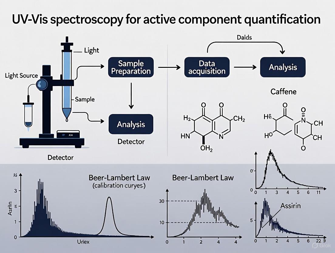
Case Study: Caffeine Quantification in Formulations

Background: Regulatory requirements mandate accurate caffeine quantification in pharmaceutical formulations, with legal limits on caffeine content that must be accurately represented on product labels [1].

Methodology:

• Extraction of caffeine from matrix using appropriate solvent
• Scanning from 200-400 nm to identify caffeine absorbance maximum (~273 nm)
• Preparation of caffeine standards in concentration range 2-20 μg/mL
• Measurement of unknown samples against calibration curve

Results Interpretation:

• Absorbance values of unknown samples fitted to linear regression equation
• Concentration calculation considering appropriate dilution factors
• Comparison against regulatory limits with ±5% accuracy requirement

Quality Control Application:

• Routine analysis of production batches for compliance verification
• Stability testing to monitor potency over shelf life
• Formulation development to optimize caffeine concentration

Troubleshooting and Method Validation

Successful implementation of UV-Vis spectroscopy for active component quantification requires awareness of potential limitations and implementation of appropriate validation protocols.

Common Limitations and Solutions

Sample Limitations: UV-Vis spectroscopy works optimally with liquids and solutions, while suspensions of solid particles can scatter light more than absorb it, skewing data [5]. Solutions include:

• Filtration or centrifugation to remove particulate matter
• Use of integrating sphere accessories for scattering samples
• Appropriate sample dilution to minimize inner filter effects

Solvent Selection: Solvents must be transparent in the spectral region of interest. Common solvent cutoffs include:

• Water: 190 nm
• Acetonitrile: 190 nm
• Methanol: 205 nm
• Chloroform: 240 nm
• Dimethyl sulfoxide: 260 nm

Stray Light Effects: Stray light reaching the detector without passing through the sample causes deviation from Beer-Lambert law at high absorbances (>1.5 AU). Maintenance of instrument optical components and proper wavelength calibration minimize these effects.

Method Validation Parameters

For regulatory compliance in pharmaceutical analysis, UV-Vis methods require comprehensive validation including:

• Linearity: Demonstrated across specified concentration range with R² ≥ 0.995
• Accuracy: Recovery of 98-102% for quality control samples
• Precision: Relative Standard Deviation ≤ 2% for repeatability
• Specificity: Ability to unequivocally assess analyte in presence of expected impurities
• Limit of Detection (LOD): Typically signal-to-noise ratio of 3:1
• Limit of Quantification (LOQ): Typically signal-to-noise ratio of 10:1 with precision ≤ 5% RSD
• Robustness: Capacity to remain unaffected by small, deliberate variations in method parameters

UV-Vis spectroscopy remains a cornerstone analytical technique in pharmaceutical research and development, providing crucial data for active component quantification from discovery through quality control. The fundamental principles of electronic transitions, chromophore absorption, and the Beer-Lambert law create a robust foundation for quantitative analysis. When implemented with proper experimental protocols, calibration procedures, and validation protocols, UV-Vis spectroscopy delivers reliable, accurate, and precise results essential for drug development.

The continuing relevance of UV-Vis spectroscopy in modern laboratories is assured by its unique combination of simplicity, cost-effectiveness, and versatility. For researchers and drug development professionals, mastery of both the theoretical principles and practical applications contained in this document provides an essential skill set for successful pharmaceutical analysis. As technology advances, the integration of UV-Vis spectroscopy with automated platforms and data analytics continues to expand its utility in the rapidly evolving pharmaceutical landscape.

Ultraviolet-Visible (UV-Vis) spectroscopy serves as a fundamental analytical technique in pharmaceutical research and drug development, providing a robust means for the identification and quantification of active pharmaceutical ingredients (APIs). This technique operates on the principle of measuring the absorption of light in the ultraviolet (190-400 nm) and visible (400-800 nm) regions of the electromagnetic spectrum, which corresponds to the excitation of electrons to higher energy states [7]. The instrumentation's core components work in concert to deliver precise, reproducible data essential for compliance with rigorous regulatory standards. The quantification capability stems primarily from the Beer-Lambert Law (A = εcl), which establishes a linear relationship between absorbance (A) and the concentration (c) of the analyte in a solution [8] [7]. This application note provides a detailed breakdown of the key instrumental components—light sources, monochromators, and detection systems—and outlines standardized protocols for their application in quantifying active components, framed within the context of analytical research for drug development.

Core Instrumentation Components

The performance, accuracy, and sensitivity of a UV-Vis spectrophotometer are determined by the integrated operation of its three key subsystems: the light source, the wavelength selection system, and the detector.

A stable light source capable of emitting consistent intensity across a broad wavelength range is fundamental. Spectrophotometers typically use multiple lamps to cover the entire UV-Vis spectrum effectively [9] [8].

Table 1: Characteristics of Common UV-Vis Light Sources

Light Source	Spectral Range	Key Characteristics	Pharmaceutical Application Suitability
Deuterium Lamp	190 - 350 nm [9]	Intense, continuous spectrum in the UV region; lifetime is a key consideration.	Ideal for quantifying APIs with chromophores absorbing in the deep UV range.
Tungsten-Halogen Lamp	330 - 2500 nm [9] [10]	Robust, long-lasting, and cost-effective for the visible to NIR region.	Suitable for colored compounds or formulation assays using visible wavelengths.
Xenon Lamp	190 - 800 nm [10] [8]	Covers both UV and Vis with a single lamp; higher cost and can be less stable.	Useful for rapid scanning across a wide range but may require more frequent calibration.

Modern instruments automatically switch between the deuterium and tungsten-halogen lamps during a scan, with the transition typically engineered to occur smoothly between 300 and 350 nm where their light emission is comparable [8] [7].

Wavelength Selection: Monochromators

The monochromator is critical for selecting discrete wavelengths from the broad-spectrum light source to probe specific electronic transitions of a sample's chromophores. Its primary function is to disperse the light and select a narrow band of wavelengths to irradiate the sample [9] [10]. The core components include an entrance slit, a collimating mirror, a dispersing element (usually a diffraction grating), a focusing mirror, and an exit slit [9].

The diffraction grating, characterized by its groove frequency (grooves per mm), is rotated to select specific wavelengths. A higher groove frequency (e.g., 1200 grooves/mm or more) provides better optical resolution [8]. The width of the exit slit determines the Spectral Bandwidth (SBW), defined as the full width at half maximum (FWHM) of the light intensity distribution [9]. A narrower SBW provides better resolution, allowing for the differentiation of sharp absorption peaks, which is crucial for identifying specific APIs in a mixture. Conversely, a wider SBW allows more light to reach the detector, improving the signal-to-noise ratio, which can be beneficial for measuring highly scattering samples or low concentrations [9]. The optimal bandwidth is typically set to 1/10 of the natural width of the sample's absorption peak [9].

Detection Systems

The detector converts the transmitted light intensity into an electrical signal, which is then processed to generate the absorption spectrum. The choice of detector impacts the sensitivity, wavelength range, and signal-to-noise ratio of the measurement [9] [8].

Table 2: Comparison of UV-Vis Spectrophotometer Detectors

Detector Type	Operating Principle	Wavelength Range	Advantages	Limitations
Photomultiplier Tube (PMT)	Photoelectric effect with amplification via dynodes [9] [10]	UV-Vis	Very high sensitivity and low noise; excellent for low-light applications [9].	Can be damaged by intense light; limited dynamic range [10].
Silicon Photodiode	Semiconductor generates current when photons are absorbed [9]	~190 - 1100 nm [10]	Robust, fast response time, wide dynamic range, and cost-effective [9].	Generally less sensitive than PMT [9].
Photodiode Array (PDA)	Array of individual photodiodes allowing simultaneous multi-wavelength detection [10]	UV-Vis	Extremely fast acquisition, enabling real-time monitoring of reactions [10].	Resolution and sensitivity can be lower than a PMT-based system.

Experimental Protocols for Active Component Quantification

Protocol: Quantification of an Active Pharmaceutical Ingredient (API)

This protocol details the use of UV-Vis spectrophotometry for the absolute quantification of a single API in a standard solution.

1. Principle: The concentration of an API in solution is determined by measuring its absorbance at a wavelength of maximum absorption (λmax) and applying the Beer-Lambert Law. A calibration curve of absorbance versus concentration is constructed using standard solutions of known concentration [7].

2. Research Reagent Solutions: Table 3: Essential Materials for API Quantification

Item	Specification	Function
UV-Vis Spectrophotometer	Double-beam configuration recommended	Compensates for source drift and solvent absorption [9].
Cuvettes	Quartz, 1 cm path length	Transparent across the entire UV-Vis range [8].
API Standard	Certified Reference Material (CRM), high purity	Used to prepare calibration standards for accurate quantification.
Solvent	UV-grade (e.g., methanol, water, buffer)	Dissolves the analyte and must not absorb significantly at the λmax [7].
Volumetric Flasks	Class A	For accurate preparation of standard and sample solutions.
Micropipettes	Calibrated	For precise liquid handling.

3. Methodology:

• Instrument Setup and Blank Measurement: Turn on the instrument and allow the lamps to stabilize for at least 30 minutes. Set the desired instrumental parameters (e.g., wavelength range, SBW). Fill a cuvette with the pure solvent and place it in the reference cell holder. Place an identical empty cuvette in the sample holder and run a baseline correction to account for solvent absorption [8].
• Preparation of Standard Solutions: Accurately weigh the API standard. Dissolve and dilute to prepare a stock standard solution. Serially dilute the stock solution with the solvent to prepare at least five standard solutions covering a concentration range where absorbance remains linear (typically Abs < 1.0) [8].
• Determination of λmax: Scan one of the standard solutions (e.g., a mid-range concentration) over a suitable wavelength range to obtain its absorption spectrum. Identify the wavelength of maximum absorption (λmax).
• Measurement of Standards and Sample: Set the spectrophotometer to the fixed λmax. Measure the absorbance of each standard solution and the unknown sample solution in triplicate. Always use the solvent blank to zero the instrument before measurements.
• Data Analysis and Calculation: Plot the average absorbance of the standard solutions against their known concentrations to generate a calibration curve. Perform linear regression analysis. The equation of the line (y = mx + c, where y is absorbance and x is concentration) is used to calculate the concentration of the API in the unknown sample based on its measured absorbance.

Protocol: Purity Assessment of Nucleic Acids for Biopharmaceuticals

In the development of nucleic acid-based therapeutics, assessing the purity of DNA or RNA preparations is a critical quality control step.

1. Principle: The concentration and purity of nucleic acid samples are determined by measuring their absorbance at specific wavelengths. The absorbance at 260 nm is proportional to the concentration of nucleic acids. The ratio of absorbance at 260 nm to 280 nm (A260/A280) is used to assess protein contamination, while the A260/A230 ratio indicates contamination by solvents or salts [7].

2. Methodology:

• Instrument Preparation: Use a double-beam spectrophotometer. Zero the instrument using a cuvette filled with the dilution buffer (e.g., Tris-EDTA buffer).
• Sample Preparation: Dilute the nucleic acid sample appropriately with the same buffer. A typical dilution for DNA is 1:100 to ensure the A260 reading is between 0.1 and 1.0.
• Measurement: Measure the absorbance of the diluted sample at 230 nm, 260 nm, and 280 nm.
• Data Analysis and Interpretation:
  • Concentration: For double-stranded DNA, Concentration (ng/μL) = A260 × 50 × Dilution Factor.
  • Purity Ratios: Interpret the results as follows:
    • Pure DNA: A260/A280 ratio ~1.8 [7].
    • Pure RNA: A260/A280 ratio ~2.0 [7].
    • Acceptable A260/A230 ratio: Typically >2.0 for both DNA and RNA [7].
  • Significant deviation from these ratios suggests contamination that may interfere with downstream enzymatic processes or analytical methods.

Instrumental Workflow and Signaling Pathways

The following diagram illustrates the logical sequence and component interaction within a standard double-beam UV-Vis spectrophotometer, which is the preferred configuration for high-precision quantitative analysis.

Diagram 1: Logical workflow of a double-beam UV-Vis spectrophotometer.

Critical Considerations for Analytical Performance

Stray Light and Photometric Linearity

Stray light, defined as any light reaching the detector that is outside the selected wavelength band, is a primary factor compromising photometric accuracy, particularly at high absorbances [9]. It causes a negative deviation from the Beer-Lambert Law, resulting in measured absorbances that are lower than the true value. This directly impacts the photometric linearity of the instrument—the range over which absorbance readings are accurately proportional to concentration [9]. For assays requiring high accuracy at elevated concentrations, instruments with double monochromators can be employed to minimize stray light.

Solvent and Cuvette Selection

The choice of solvent and cuvette material is critical:

• Solvents must be transparent in the spectral region of interest. Common solvents for UV-Vis include water, hexane, 95% ethanol, and methanol [7].
• Cuvettes must be selected based on the wavelength range. Standard quartz or fused silica cuvettes are required for UV work (down to 190 nm), while glass or plastic may be suitable for visible-only measurements [8].

A detailed understanding of UV-Vis instrumentation—from the characteristics of light sources and the resolution of monochromators to the sensitivity of detection systems—is paramount for researchers and scientists engaged in the quantification of active components. The precise and robust protocols outlined for API quantification and nucleic acid purity analysis provide a framework for generating reliable, reproducible data essential for drug development pipelines. By adhering to these standardized methodologies and being mindful of critical factors such as spectral bandwidth and stray light, professionals can ensure the integrity of their analytical results, thereby supporting the development of safe and effective pharmaceutical products.

Ultraviolet-Visible (UV-Vis) spectroscopy is an instrumental analytical technique that measures the absorption of light by a chemical substance in the ultraviolet (typically 100-400 nm) and visible (400-800 nm) regions of the electromagnetic spectrum [11] [12]. This measurement occurs when valence electrons in molecules are promoted from their ground state to higher energy excited states by absorbing specific wavelengths of light [12]. The technique is widely employed across scientific disciplines due to its relative simplicity, cost-effectiveness, non-destructive nature, and rapid analysis capabilities [2].

The quantitative application of UV-Vis spectroscopy fundamentally relies on the Beer-Lambert Law (also known as Beer's Law) [13] [14]. This law establishes the foundational relationship between the amount of light absorbed by a solution and the concentration of the absorbing species within it, thereby enabling researchers to precisely quantify analytes [15]. The combined Beer-Lambert Law provides the mathematical basis for modern spectrophotometric analysis, making it indispensable for drug development and analytical research.

Theoretical Foundation of the Beer-Lambert Law

The Beer-Lambert Law synthesizes two historical observations: Lambert's law, which states that absorbance is proportional to the path length of the light through the sample, and Beer's law, which states that absorbance is proportional to the concentration of the absorbing species [14] [15]. The unified law is expressed by the equation:

A = ε * c * l

Where:

• A is the Absorbance (also known as optical density), a dimensionless quantity defined as A = log₁₀(Iâ‚€/I) [14] [11]. Here, Iâ‚€ is the intensity of the incident light, and I is the intensity of the transmitted light.
• ε is the Molar Absorptivity (or molar extinction coefficient), with typical units of L·mol⁻¹·cm⁻¹ [15]. This is a characteristic constant for a given substance at a specific wavelength, measuring the probability of electronic transitions [14].
• c is the Molar Concentration of the absorbing solute in the solution, with units of mol·L⁻¹ [15].
• l is the Path Length, representing the distance (in cm) the light travels through the sample [15].

Mathematical Derivation and Key Relationships

The derivation of the Beer-Lambert Law begins with the observation that the decrease in light intensity (-dI) across an infinitesimally thin layer of solution (dx) is proportional to the incident intensity (I), the concentration of the absorber (c), and the thickness of the layer [14].

• This relationship is expressed as: -dI/dx = α * I * c, where α is a proportionality constant.
• Integrating this differential equation and applying the boundary condition that I = Iâ‚€ when x = 0 yields: ln(Iâ‚€/I) = α * c * x.
• Converting the natural logarithm to base-10 gives: log₁₀(Iâ‚€/I) = (α/2.303) * c * x.
• By defining Absorbance A = log₁₀(Iâ‚€/I) and substituting the molar absorptivity ε for (α/2.303), the final form is obtained: A = ε * c * l [14] [15].

This derivation confirms the linear relationship between absorbance and concentration, which is the cornerstone of quantitative analysis.

Quantitative Data and Units

The following table summarizes the core components and their standard units in the Beer-Lambert equation.

Table 1: Core Components of the Beer-Lambert Law and Their Standard Units

Quantity	Symbol	Formula	Units
Absorbance	A	A = log₁₀(I₀/I)	None (dimensionless)
Molar Absorptivity	ε	In A = ε c l	L·mol⁻¹·cm⁻¹
Concentration	c	In A = ε c l	mol·L⁻¹
Path Length	l	In A = ε c l	cm

Applications in Analytical Research

The Beer-Lambert Law is the driving principle behind countless quantitative analyses in research and industry. Its primary application is determining the concentration of an unknown sample by measuring its absorbance and applying the law, either directly or via a calibration curve [12].

DNA and RNA Quantification

In molecular biology and genetics, quantifying nucleic acids is a critical step. The concentration of pure double-stranded DNA (dsDNA) can be determined directly using its absorbance at 260 nm. An absorbance of 1.0 at 260 nm corresponds to approximately 50 µg/mL of dsDNA [16]. The calculation is:

Concentration (µg/mL) = A₂₆₀ reading × Dilution Factor × 50 µg/mL

Purity is assessed using absorbance ratios. For pure DNA, the A₂₆₀/A₂₈₀ ratio should be between 1.8 and 2.0. A lower ratio suggests protein contamination (as proteins absorb at 280 nm). The A₂₆₀/A₂₃₀ ratio, which should be greater than 1.5, indicates contamination by organic compounds or chaotropic salts [16].

Protein Quantification via A₂₈₀ Absorbance

Protein concentration can be estimated by measuring absorbance at 280 nm, which is primarily due to the aromatic amino acids tryptophan and tyrosine [17]. This method is quick and simple, as it requires no additional reagents. The measurable concentration range for Bovine Serum Albumin (BSA) using this direct absorbance method is approximately 125-1000 µg/mL [17]. While convenient, this method's accuracy can be affected by the specific aromatic amino acid composition of the protein.

Determination of Unknown Concentrations Using a Calibration Curve

For most accurate results, especially with complex matrices or when the exact molar absorptivity is unknown, a calibration curve is constructed [12]. This procedure involves:

• Preparing a series of standard solutions with known concentrations of the analyte.
• Measuring the absorbance of each standard at a specific wavelength (preferably at λ_max, the wavelength of maximum absorption).
• Plotting absorbance versus concentration to create a scatter plot.
• Fitting a straight line (using linear regression) to the data points.

The equation of this line (y = mx + b, where y is absorbance and x is concentration) is then used to calculate the concentration of an unknown sample from its measured absorbance [18]. This approach empirically accounts for the specific experimental conditions and is considered more reliable than relying on a literature value for ε.

Detailed Experimental Protocols

Protocol 1: Quantifying DNA Concentration and Purity by UV Absorbance

This protocol is used for the rapid quantification and purity assessment of purified DNA samples [16].

The Scientist's Toolkit: Research Reagent Solutions

• DNA Sample: The nucleic acid to be quantified.
• TE Buffer or Nuclease-Free Water: A blank solution to dilute the DNA and serve as the reference. It must be UV-transparent.
• Quartz Cuvette: For holding the sample during measurement. Quartz is required for UV light transmission.
• UV-Vis Spectrophotometer: The instrument capable of generating and measuring light in the UV range.

Procedure:

• Blank Measurement: Pipette an appropriate volume of the blank solution (e.g., TE buffer) into a quartz cuvette and place it in the spectrophotometer. Perform a blank measurement to calibrate the instrument to 100% transmittance / 0.000 absorbance.
• Sample Preparation: Dilute the DNA sample with the same blank solution. A typical dilution factor for concentrated DNA is 1:50 or 1:100.
• Absorbance Measurement: Measure the absorbance of the diluted DNA sample at 230 nm, 260 nm, and 280 nm.
• Data Analysis:
  • Concentration Calculation: dsDNA Concentration (ng/µL) = A₂₆₀ × Dilution Factor × 50.
  • Purity Assessment: Calculate the A₂₆₀/A₂₈₀ and A₂₆₀/A₂₃₀ ratios.

DNA Quantification Workflow

Protocol 2: Determining Protein Concentration by A₂₈₀ Absorbance

This protocol is suitable for a quick estimation of protein concentration, provided the sample is pure and the buffer does not contain strong UV-absorbing additives [17].

The Scientist's Toolkit: Research Reagent Solutions

• Protein Sample: The protein solution to be quantified.
• Reference Buffer: The exact buffer the protein is dissolved in, used for blanking.
• Quartz Cuvette: Essential for UV measurements at 280 nm.
• UV-Vis Spectrophotometer: The instrument for absorbance measurement.

Procedure:

• Blank Measurement: Pipette the reference buffer into a quartz cuvette and blank the spectrophotometer at 280 nm.
• Sample Measurement: Replace the blank with the protein sample and measure the absorbance at 280 nm. Ensure the absorbance reading is within the linear range of the instrument (preferably between 0.1 and 1.5 AU). If it is too high, dilute the sample and re-measure.
• Concentration Calculation: Use the protein-specific molar absorptivity (ε) or the general approximation for IgG antibodies (A₂₈₀ of 1.4 ≈ 1 mg/mL). Alternatively, construct a calibration curve using a standard like BSA for greater accuracy.

Table 2: Comparison of Absorbance-Based Protein Quantification Methods

Method	Principle	Wavelength (nm)	Typical Range (µg/mL)	Advantages	Disadvantages
Direct A₂₈₀	Absorption by Trp/Tyr residues	280	125 - 1000 [17]	Fast, no reagents, sample recoverable	Affected by buffer composition; less accurate
Bradford Assay	Coomassie dye binding shift	595 (from 465) [17]	62.5 - 1000 [17]	Sensitive, simple protocol	Non-linear response; dye interference
BCA Assay	Cu²⁺ reduction by peptides	562 [17]	15.6 - 1500 [17]	Tolerant to some detergents; sensitive	Time-consuming (30 min incubation)

Critical Considerations and Limitations

Despite its widespread utility, the Beer-Lambert Law is subject to deviations under non-ideal conditions. Researchers must be aware of these limitations to ensure accurate data interpretation.

Fundamental Conditions for Valid Application

For the Beer-Lambert Law to hold true, several conditions must be met [14] [15]:

• Monochromicity of Light: The incident light should be monochromatic. The use of polychromatic light can lead to negative deviations from the law [11].
• Low Concentration: The absorbing species must be at a relatively low concentration. At high concentrations (>0.01 M), electrostatic interactions between molecules can alter the absorptivity [14] [15].
• Chemical Independence: The absorbers must act independently of one another. Chemical phenomena such as association, dissociation, or polymerization in response to concentration changes will cause deviations [15].
• Homogeneous Sample: The sample must be a homogeneous solution without turbidity. Scattering due to particles, bubbles, or colloids will falsely increase the measured absorbance [12].
• Stray Light: Stray light within the spectrophotometer, which is light of wavelengths outside the band selected by the monochromator, can cause significant errors, particularly at high absorbances, leading to a plateau in the calibration curve [11].

Real-World Deviations and Nonlinearity

In practice, deviations from the linear Beer-Lambert relationship are common. A 2022 study highlighted the widespread misuse of calibration curves, emphasizing that the classical method of regressing concentration on absorbance is statistically incorrect; the proper inverse regression (absorbance on concentration) should be used for predicting unknown concentrations [18]. Furthermore, a 2021 empirical investigation found that while high concentrations of lactate (up to 600 mmol/L) did not introduce significant nonlinearities, highly scattering media (like whole blood) did justify the use of more complex, nonlinear models [19]. This underscores the importance of matching the analytical method to the sample matrix.

Ultraviolet-visible (UV-Vis) spectroscopy is a fundamental analytical technique in research and drug development for the identification and quantification of active components. Its operation is grounded in the Beer-Lambert Law, which establishes that the absorbance of a solution is directly proportional to the concentration of the absorbing species (the analyte), its molar absorptivity, and the path length of light through the sample [12]. The accurate quantification of any analyte therefore hinges on the precise understanding and control of three essential parameters: the wavelength of measurement, the molar absorptivity of the analyte, and the path length of the sample container. This document provides detailed application notes and protocols to guide researchers in optimizing these parameters for robust and reliable quantitative analysis.

Core Principles and the Beer-Lambert Law

The foundational relationship for quantitative UV-Vis spectroscopy is the Beer-Lambert Law, expressed as:

A = εcl

Where:

• A is the measured Absorbance (dimensionless) [8]
• ε is the Molar Absorptivity (or molar extinction coefficient) with units of L·mol⁻¹·cm⁻¹ [20] [12]
• c is the Molar Concentration of the absorber (mol·L⁻¹)
• l is the Path Length of the light through the sample (cm) [12]

This linear relationship allows for the direct determination of an unknown concentration once the absorbance, path length, and molar absorptivity are known [12] [11]. The following sections delve into the critical considerations for each of these parameters.

Parameter 1: Wavelength Selection

The choice of wavelength is critical for achieving maximum sensitivity, selectivity, and adherence to the Beer-Lambert Law.

Optimal Wavelength Criteria

The primary criterion for quantitative analysis is to select the wavelength at which the analyte has the highest molar absorptivity, known as λmax (lambda max) [21] [22]. Measuring at λmax provides the greatest analytical sensitivity, as the largest absorbance signal is obtained for a given concentration, which improves the signal-to-noise ratio. Furthermore, the absorption spectrum is typically flattest near the peak, meaning that the molar absorptivity changes least with small, inevitable drifts in the instrument's wavelength calibration. This minimizes errors in concentration calculations [11].

Table 1: Characteristic Absorption Maxima for Common Chromophores

Chromophore / Functional Group	Electronic Transition	Typical λ_max Range (nm)	Molar Absorptivity (ε) Range (L·mol⁻¹·cm⁻¹)
Carbonyl (C=O)	n → π*	270 - 300	10 - 100 [20]
Aromatic Systems	π → π*	250 - 280	~200 - 10,000 [20]
Conjugated Dienes	π → π*	220 - 250	~10,000 - 25,000 [20]
Highly Conjugated Systems	π → π*	>300	Can exceed 50,000 [20]

Protocol for Wavelength Selection and Verification

Methodology:

• Preliminary Scan: Prepare a standard solution of the pure analyte within the concentration range expected for your samples. Using a spectrophotometer, perform a full wavelength scan (e.g., from 200 nm to 800 nm, or a relevant range for the analyte) against a solvent blank [22].
• Identify λmax: From the resulting absorption spectrum, identify the wavelength corresponding to the highest absorbance peak. This is the preliminary λmax [22].
• Check for Interferences: Prepare a blank matrix that mimics the sample but lacks the analyte. Scan this solution over the same wavelength range. If the blank shows significant absorption at the chosen λ_max, consider using an alternative, secondary absorption peak where interference is minimal, even if the molar absorptivity is lower [21].
• Final Method Validation: The selected wavelength must be validated as part of the overall analytical method to ensure specificity, accuracy, and precision.

Parameter 2: Molar Absorptivity

Molar absorptivity (ε) is an intrinsic property of a chemical species at a given wavelength and temperature, representing its ability to absorb light [20].

Factors Influencing Molar Absorptivity

The value of ε is primarily determined by the electronic structure of the molecule. Key influencing factors include:

• Chromophore Type: Different functional groups and their associated transitions (e.g., π→π* vs. n→π) have characteristic and vastly different absorptivities. For instance, π→π transitions are typically "allowed" and have high ε values (often >10,000), whereas n→π* transitions are "forbidden" and have low ε values (typically 10-100) [20] [22].
• Conjugation: Extending conjugation in a molecule (e.g., in polyenes or aromatic systems) delocalizes electrons, lowers the energy required for electronic transition, and results in a bathochromic (red) shift to longer wavelengths along with a hyperchromic effect (increase in ε) [20]. This is a key design principle for creating highly sensitive assays.
• Solvent and Environment: Solvent polarity can cause shifts in λ_max and changes in ε, particularly for transitions involving non-bonding electrons (n→π). Protic solvents can hydrogen-bond to n electrons, stabilizing the ground state and increasing the energy required for an n→π transition, leading to a hypsochromic (blue) shift and potential change in ε [20]. pH can also dramatically affect the absorption profile of ionizable chromophores [21].

Protocol for Determining Molar Absorptivity

Methodology:

• Prepare Standard Solutions: Accurately prepare a series of at least five standard solutions of the analyte with known concentrations, spanning the expected working range. The concentrations should be chosen such that the measured absorbance values fall within the linear range of the instrument, ideally between 0.1 and 1.0 AU [22].
• Measure Absorbance: Measure the absorbance of each standard solution at the predetermined λ_max, using the appropriate solvent as a blank. Ensure a fixed, known path length (e.g., 1 cm) [22].
• Construct Calibration Curve: Plot the measured absorbance (y-axis) against the corresponding concentration (x-axis).
• Calculate Molar Absorptivity: Perform linear regression on the data. The slope of the resulting calibration curve is equal to the product of the molar absorptivity and the path length (slope = εl). Since the path length (l) is known (e.g., 1 cm), the molar absorptivity (ε) can be calculated directly from the slope [12] [22].

Parameter 3: Path Length

The path length (l) is the distance the light travels through the sample solution. According to the Beer-Lambert Law, absorbance is directly proportional to path length for a given concentration [12].

Path Length Considerations and Linearity

Standard cuvettes have a path length of 1.0 cm. However, a variety of path lengths are available and can be selected based on the sample concentration:

• High Concentration Samples: For highly absorbing samples, a shorter path length (e.g., 0.1 cm or 1 mm) can be used to bring the absorbance reading back into the optimal range of 0.1-1.0 AU, thereby avoiding deviations from the Beer-Lambert Law [8].
• Low Concentration Samples: For very dilute solutions, a longer path length (e.g., 2 cm, 5 cm, or 10 cm) can be used to increase the absorbance signal and improve detection limits.
• Linearity Verification: A key test for the validity of the Beer-Lambert Law for a given system is to demonstrate that absorbance is linearly proportional to path length. This can be tested by measuring the same sample in cuvettes of different path lengths; a plot of absorbance vs. path length should yield a straight line [11].

Integrated Workflow for Method Development

The following diagram and protocol outline a systematic approach for developing a quantitative UV-Vis method, integrating the three essential parameters.

Diagram 1: UV-Vis Quantification Method Workflow

Comprehensive Experimental Protocol for Active Component Quantification

Objective: To quantify the concentration of an active pharmaceutical ingredient (API) in a solution.

Materials:

• The Scientist's Toolkit: Key Research Reagent Solutions
  • High-Purity Reference Standard: The authentic, high-purity analyte for preparing calibration standards [11].
  • Appropriate Solvent: A solvent that dissolves the analyte and does not absorb significantly in the spectral region of interest (e.g., water, methanol, acetonitrile) [8] [22].
  • Volumetric Flasks: For accurate preparation and dilution of standard and sample solutions.
  • Matched Cuvettes: A pair of spectrometric cuvettes with a known, fixed path length (e.g., 1 cm). For UV work, quartz cuvettes are required; glass or plastic may be used for visible light only [8].
  • Micropipettes: For accurate and precise liquid handling.
  • UV-Vis Spectrophotometer: A calibrated instrument with a scanning capability.

Procedure:

• Solution Preparation:
  • Stock Standard Solution: Accurately weigh the reference standard and dissolve it in the chosen solvent to prepare a stock solution of known concentration.
  • Calibration Standards: Serially dilute the stock solution with solvent to prepare at least five standard solutions covering a concentration range that will produce absorbances between 0.1 and 1.0 AU.
  • Sample Solution: Prepare the unknown sample by dissolving or diluting it in the same solvent to bring its expected concentration within the range of the calibration standards.

• Spectrophotometric Analysis:

  • Turn on the UV-Vis spectrophotometer and allow it to warm up as per the manufacturer's instructions.
  • Set the instrument to measure absorbance.
  • Fill a cuvette with the pure solvent (the "blank"), place it in the sample holder, and perform a blank correction.
  • For wavelength selection (Diagram 1, Box P1), replace the blank with an intermediate standard solution and perform a full wavelength scan to identify and confirm the λ_max for the analyte.
  • For quantification (Diagram 1, Boxes P2 & P3), set the instrument to the fixed λ_max. Measure the absorbance of each calibration standard and the unknown sample solution against the solvent blank. Ensure all measurements are performed using the same cuvette or matched cuvettes with the same path length.

• Data Analysis and Calculation:

  • Plot a calibration curve with absorbance on the y-axis and standard concentration on the x-axis.
  • Perform a linear regression analysis to obtain the equation of the line (y = mx + b, where y is absorbance and x is concentration) and the correlation coefficient (R²).
  • The slope (m) of the line is equal to εl. If the path length (l) is 1 cm, the slope is the molar absorptivity (ε).
  • Substitute the absorbance of the unknown sample (y) into the linear equation and solve for the concentration (x).

Troubleshooting and Best Practices

• Deviations from Beer-Lambert Law: Non-linearity can occur at high concentrations (>0.01 M) due to electrostatic interactions or changes in refractive index [20]. It can also be caused by instrumental factors such as stray light, which becomes significant at high absorbances (typically >1.0 AU) and leads to a false lower absorbance reading [11].
• Stray Light Mitigation: Use a spectrophotometer with a low stray light specification and ensure concentrations/path lengths are chosen to keep absorbance readings below 1.0-1.5 AU for quantitative work [11].
• Sample Preparation Errors: Ensure samples are fully dissolved and free of bubbles or particulate matter that can scatter light and cause erroneously high absorbance readings [12] [22]. Always use clean, scratch-free cuvettes.

By systematically applying these principles and protocols, researchers can develop validated, robust, and reliable UV-Vis spectroscopic methods for the accurate quantification of active components in pharmaceutical research and development.

Ultraviolet-visible (UV-Vis) spectroscopy is a cornerstone analytical technique in pharmaceutical laboratories due to its inherent advantages in speed, cost-effectiveness, and accuracy. This application note details how these benefits are realized in the quantification of active pharmaceutical ingredients (APIs), supported by structured experimental protocols. Framed within broader research on API quantification, this document provides scientists and drug development professionals with validated methodologies that align with regulatory standards, including United States (USP), European (EP), and Japanese (JP) pharmacopeias [23].

UV-Vis spectroscopy measures the absorption of discrete wavelengths of ultraviolet or visible light by a sample. The fundamental principle is governed by the Beer-Lambert Law (A = εlc), which states that absorbance (A) is proportional to the concentration (c) of the analyte, its molar absorptivity (ε), and the path length (l) of light through the sample [8] [24]. This direct relationship provides the foundation for its quantitative use in pharmaceutical analysis. The technique is versatile, supporting applications from drug discovery and development to quality control (QC) and impurity profiling [23]. Its compliance with international pharmacopeias makes it an indispensable tool for regulated laboratories.

Core Advantages in Pharmaceutical Analysis

The deployment of UV-Vis spectroscopy in the pharmaceutical industry is driven by three principal advantages, summarized in the table below.

Table 1: Key Advantages of UV-Vis Spectroscopy in Pharmaceutical Analysis

Advantage	Description	Impact in Pharmaceutical Context
Speed	Delivers results in minutes or even seconds; requires minimal sample preparation [24].	Accelerates high-throughput screening in drug discovery and enables rapid quality control (QC) release of finished products [23].
Cost-Effectiveness	Lower initial instrument cost and maintenance compared to techniques like HPLC or MS; minimal consumable use (e.g., quartz cuvettes) [24].	Reduces overall analytical costs for both research and development (R&D) and QC laboratories, making it accessible for various levels of operation.
Accuracy & Precision	Provides highly accurate and precise quantitative results when properly calibrated and validated; compliant with pharmacopeial standards for identity, assay, and purity [23].	Ensures reliability of data for regulatory submissions and guarantees that APIs and finished products meet stringent quality specifications.

These advantages are synergistic. The speed and low cost allow for frequent testing and monitoring, while the inherent accuracy ensures the data generated is reliable for critical decision-making throughout the drug development lifecycle.

Essential Research Toolkit

Successful implementation of UV-Vis protocols requires specific instrumentation and reagents. The following table lists the essential components for a pharmaceutical analysis laboratory.

Table 2: Key Research Reagent Solutions and Essential Materials

Item	Function/Description
UV-Vis Spectrophotometer	An instrument with a deuterium (UV) and tungsten/halogen (Vis) lamp source, capable of scanning from ~190 nm to 800 nm. Models with regulated software (e.g., for 21 CFR Part 11 compliance) are essential for QC [23].
Quartz Cuvettes	Sample holders transparent to UV light. Glass or plastic cuvettes are unsuitable for UV range measurements as they absorb UV light [8].
Reference Solvent	A high-purity solvent (e.g., the same buffer used to dissolve the sample) to zero the instrument and establish a baseline absorbance [8].
Pharmaceutical Standards	Certified Reference Materials (CRMs) of the target Active Pharmaceutical Ingredient (API) with known purity and concentration for calibration [23].
Volumetric Glassware	Precise flasks and pipettes for accurate sample and standard solution preparation.
N,N-dimethylhex-5-ynamide	N,N-dimethylhex-5-ynamide
1-methyl-1H-indole-2-thiol	1-Methyl-1H-indole-2-thiol

Application Notes & Experimental Protocols

Protocol 1: Quantitative Analysis of an Active Pharmaceutical Ingredient (API)

This protocol outlines the steps for quantifying the concentration of an API, such as ibuprofen, in a solution using a direct absorbance measurement [23].

Workflow Overview:

Materials:

• API reference standard
• Appropriate solvent (e.g., phosphate buffer, methanol)
• Volumetric flasks (e.g., 10 mL, 25 mL, 100 mL)
• Pipettes
• UV-Vis spectrophotometer with quartz cuvettes

Procedure:

• Solution Preparation:
  • Prepare a stock solution of the API reference standard at a known concentration (e.g., 100 µg/mL).
  • Using serial dilution, prepare a series of at least five standard solutions covering a concentration range where absorbance is linear (e.g., 5, 10, 20, 30, 40 µg/mL). Ensure absorbance values remain below 1.0 for reliability [8].
• Instrument Setup:
  • Turn on the UV-Vis spectrophotometer and allow the lamps to warm up for the time specified by the manufacturer (typically 15-30 minutes).
  • Set the instrument to the wavelength of maximum absorption (λmax) for the API, which can be determined from a preliminary scan or literature (e.g., 221 nm for ibuprofen in alkaline medium as per USP) [23].
• Blank Measurement:
  • Fill a quartz cuvette with the pure solvent used to prepare the standards and place it in the sample holder.
  • Use this measurement to zero the instrument (set absorbance to 0.0).
• Calibration Curve:
  • Measure the absorbance of each standard solution in sequence.
  • Record the absorbance values and plot a graph of absorbance (y-axis) versus concentration (x-axis). The software typically generates a linear regression equation (y = mx + c).
• Sample Analysis:
  • Prepare a sample solution of the unknown API concentration within the linear range of the calibration curve.
  • Measure its absorbance at the same λmax.
  • Use the regression equation from the calibration curve to calculate the concentration of the unknown sample.

Protocol 2: Dissolution Testing of Solid Oral Dosage Forms

Dissolution testing is critical for evaluating the release of a drug from its dosage form. UV-Vis is the standard method for analyzing the dissolved concentration in the medium [23].

Workflow Overview:

Materials:

• Dissolution test apparatus (paddles or baskets)
• Dissolution medium (e.g., buffer at pH 1.2, 4.5, or 6.8)
• Syringe filters (e.g., 0.45 µm)
• UV-Vis spectrophotometer

Procedure:

• Apparatus Setup:
  • Fill the dissolution vessel with a specified volume of pre-warmed (e.g., 37°C ± 0.5°C) dissolution medium.
  • Place the tablet or capsule into the apparatus and start the rotation at the specified speed (e.g., 50 rpm for paddles).
• Sampling:
  • At predetermined time intervals (e.g., 10, 15, 20, 30, 45, and 60 minutes), withdraw a small aliquot (e.g., 5-10 mL) from the vessel.
  • Immediately replace the withdrawn volume with fresh, pre-warmed medium to maintain a constant volume.
• Sample Preparation:
  • Filter the withdrawn aliquot through a syringe filter to remove any undissolved particles.
• Analysis:
  • Measure the absorbance of the filtered solution at the API's λmax.
  • Calculate the concentration of dissolved drug at each time point using a pre-established calibration curve (as developed in Protocol 1).
  • Report the percentage of drug released versus time to generate a dissolution profile.

Advanced Techniques: Extending Analytical Capabilities

For complex matrices, advanced UV-Vis techniques enhance the method's power and accuracy.

• Multivariate Analysis: Techniques like Principal Component Analysis (PCA) and Partial Least Squares (PLS) regression are used to extract quantitative information from spectra of complex mixtures, resolving issues like overlapping peaks from multiple analytes or excipients [24].
• Hyphenated Techniques: Coupling UV-Vis detection with High-Performance Liquid Chromatography (HPLC) creates the powerful HPLC-UV-Vis platform. Here, HPLC separates the components of a complex mixture, and the UV-Vis detector provides quantitative analysis of each separated peak, which is crucial for impurity profiling and stability-indicating methods [24].

Method Validation and Quality Assurance

To ensure data accuracy and regulatory compliance, UV-Vis methods must be validated. Key performance characteristics include:

• Linearity: Demonstrated by a high correlation coefficient (R² > 0.999) of the calibration curve.
• Accuracy: Typically confirmed through recovery studies (e.g., 98-102%).
• Precision: Evaluated as repeatability (multiple measurements of the same sample) and intermediate precision (different days, different analysts).
• Specificity: The ability to unequivocally assess the analyte in the presence of other components like impurities or excipients. This can be confirmed by comparing spectra of pure and sample solutions [23].

Regular instrument performance verification using certified reference materials (e.g., holmium oxide filters for wavelength accuracy, neutral density filters for photometric accuracy) is mandatory in pharmacopeia-compliant laboratories [23].

UV-Vis spectroscopy remains a vital analytical technique in pharmaceutical analysis due to its compelling combination of speed, cost-effectiveness, and accuracy. From straightforward API quantification to complex dissolution testing, its principles, governed by the Beer-Lambert law, provide a robust foundation for generating reliable data. When coupled with proper method validation and quality control practices, UV-Vis spectroscopy meets the stringent requirements of modern drug development and quality assurance, making it an indispensable tool in the scientist's toolkit.

Pharmaceutical Applications: From API Quantification to Dissolution Testing

Active Pharmaceutical Ingredient (API) Quantification and Purity Assessment

Ultraviolet-Visible (UV-Vis) spectroscopy serves as a cornerstone analytical technique in pharmaceutical development and quality control, enabling precise quantification of Active Pharmaceutical Ingredients (APIs) and critical assessment of their purity [25]. The technique operates on the principle of the Beer-Lambert law, which relates the absorption of light to the properties of the material through which the light is traveling [26] [24]. Its simplicity, speed, sensitivity, and cost-effectiveness make it indispensable for ensuring drug identity, potency, and stability across research, development, and manufacturing workflows [24] [27]. This application note details established protocols and methodologies for leveraging UV-Vis spectroscopy in API analysis, framed within a rigorous Analytical Quality by Design (AQbD) and method validation framework [28].

Core Principles and Method Selection

UV-Vis spectroscopy measures the absorption of light in the ultraviolet (190–380 nm) and visible (380–800 nm) regions of the electromagnetic spectrum, resulting from electronic transitions in molecules [25] [27]. The fundamental relationship between absorbance and analyte concentration is described by the Beer-Lambert Law: [A = \epsilon l c] where (A) is the measured absorbance, (\epsilon) is the molar absorptivity (a molecule-specific constant), (l) is the path length of the cuvette (cm), and (c) is the analyte concentration (mol/L) [24].

The choice of methodology depends on the analytical goal and the complexity of the sample. The table below summarizes the primary techniques used for API analysis.

Table 1: Overview of UV-Vis Techniques for API Analysis

Technique	Principle	Best Suited For	Key Advantages
Direct Quantification	Measurement of absorbance at the λₘₐₓ of a single, isolated API.	Standardized assay of pure API solutions; content uniformity [25].	Simplicity and speed.
Baseline Manipulation (Difference) Spectroscopy	Using a solution of one analyte as a blank to eliminate its spectral contribution, allowing direct measurement of a second analyte [26].	Binary mixtures in combined dosage forms without prior separation.	Eliminates need for complex separation steps; cost-effective [26].
Multivariate Analysis & Spectral Deconvolution	Application of statistical models (e.g., PLS, PCA) to extract concentration information from complex, overlapping spectra [28] [24].	Complex formulations with severe spectral overlap; in-line Process Analytical Technology (PAT) [28].	Handles complex data; enables real-time, in-line monitoring.
Hyphenated Techniques (e.g., HPLC-UV-Vis)	Coupling separation power of HPLC with the detection capability of UV-Vis [24].	Purity assessment and impurity profiling in complex mixtures.	High specificity and sensitivity; can separate and quantify multiple components.

Experimental Protocols

Protocol 1: Direct API Quantification in a Standard Solution

This fundamental protocol is used to determine the concentration of an API in a simple solution and forms the basis for many pharmacopeial methods [25].

The Scientist's Toolkit:

• UV-Vis Spectrophotometer: A double-beam instrument is preferred for stability. Must be equipped with matched quartz cuvettes (typically 1 cm path length) [26].
• High-Purity Solvent: Spectroscopic grade methanol, water, or buffer as appropriate. Must be transparent in the spectral region of interest [25].
• Analytical Balance: For precise weighing of the API standard (e.g., Shimadzu AUW-220D) [26].
• Volumetric Flasks: Class A glassware for accurate preparation of standard and sample solutions.

Step-by-Step Methodology:

• Standard Stock Solution: Accurately weigh about 100 mg of API reference standard and transfer to a 100 mL volumetric flask. Dissolve and dilute to volume with the chosen solvent to obtain a stock solution of approximately 1000 µg/mL [26].
• Working Standard Solutions: Prepare a series of working standards (e.g., 5-25 µg/mL) by precise serial dilution of the stock solution.
• Spectral Scan: Scan one of the mid-range working standards from 200 nm to 400 nm to identify the wavelength of maximum absorption (λₘₐₓ).
• Blank Preparation: Prepare a blank consisting of the pure solvent.
• Calibration Curve: Measure the absorbance of each working standard solution at the predetermined λₘₐₓ against the solvent blank. Construct a calibration curve by plotting absorbance versus concentration.
• Sample Analysis: Prepare the sample solution (e.g., from a dissolved tablet) to fall within the calibration range and measure its absorbance. Calculate the API concentration using the regression equation from the calibration curve.

Protocol 2: Purity Assessment and Contaminant Screening

UV-Vis spectroscopy can provide a rapid initial assessment of sample purity by examining the spectral profile beyond a single wavelength [29] [30].

Step-by-Step Methodology:

• Sample Preparation: Prepare a solution of the test sample at an appropriate concentration.
• Broad-Range Scanning: Record the full UV-Vis spectrum of the sample from 240 nm to 350 nm (or higher if colored) using the solvent as a blank [29].
• Spectral Analysis:
  • Check for Nucleic Acid Contamination: A distinct "bump" or elevated absorbance at ~260 nm indicates potential nucleic acid contamination. The 260/280 nm absorbance ratio should be approximately 0.57 for a pure protein; significant deviation suggests contamination [29].
  • Check for Scattering/Insolubles: A rising baseline towards lower wavelengths (particularly in the visible region) can indicate light scattering from insoluble particles or API oversaturation in a polymer matrix, as seen in Hot Melt Extrusion [28] [27].
  • Examine Peak Shape and Fine Structure: The unique microenvironment of aromatic residues in a protein confers a unique UV spectrum. Deviations from the expected spectral fine structure can indicate conformational changes or the presence of impurities [30].

Diagram: Workflow for API Analysis and Purity Assessment

Method Validation as per ICH Guidelines

For any analytical method to be used in a regulatory environment, it must be validated according to international guidelines, such as ICH Q2(R1) [26] [25]. The following table outlines key validation parameters and typical acceptance criteria for a UV-Vis method.

Table 2: Method Validation Parameters and Acceptance Criteria

Validation Parameter	Protocol Description	Typical Acceptance Criteria
Linearity & Range	Analyze a minimum of 5 concentrations in triplicate across the intended range [26].	Correlation coefficient (r) > 0.999. Fischer variance ratio test for linearity [26].
Accuracy	Perform recovery studies by spiking a placebo or pre-analyzed sample with known amounts of API at 50%, 100%, and 150% levels [26].	Mean recovery between 98.0–102.0%.
Precision	Repeatability: Six replicate analyses of a single homogenous sample [26]. Intermediate Precision: Analysis by a second analyst on a different day [26].	RSD ≤ 1.0% for repeatability. RSD ≤ 2.0% for intermediate precision.
Specificity	Demonstrate that the method can unequivocally assess the analyte in the presence of potential interferents like excipients, degradation products, or impurities [26] [25].	No interference from blank or placebo at the analyte's λₘₐₓ.
Robustness	Deliberately introduce small, purposeful variations in method parameters (e.g., wavelength ±2 nm, sonication time ±5 min) [26].	The method remains unaffected by small variations (RSD remains within specified limits).
LOD & LOQ	Calculate based on the standard deviation of the response (σ) and the slope of the calibration curve (b): LOD = 3.3σ/b; LOQ = 10σ/b [26].	Signal-to-noise ratio of 3:1 for LOD and 10:1 for LOQ.

Advanced Applications in Pharmaceutical Development

In-line Monitoring Using Process Analytical Technology (PAT)

UV-Vis spectroscopy is a powerful PAT tool for real-time monitoring of Critical Quality Attributes (CQAs) during continuous manufacturing processes like Hot Melt Extrusion (HME) [28] [27]. AQbD principles are applied to develop robust in-line methods, where an Analytical Target Profile (ATP) is established upfront. For example, in-line UV-Vis has been successfully used to monitor the API content and color (as lightness, L*) of piroxicam in a polymer melt during HME, enabling real-time release testing (RTRT) [28]. The method's validation, based on accuracy profile strategy, showed that 95% β-expectation tolerance limits were within the ±5% acceptance limits, proving its suitability for in-process control [28].

Drug Stability Testing

UV-Vis spectrophotometry is extensively used in forced, accelerated, and real-time stability studies to predict the commercial viability of drug products [31]. By subjecting drugs to stressors like light, temperature, and pH changes, scientists can track decreases in API potency (via reduced absorbance at λₘₐₓ) and the formation of degradation products (via new absorbance peaks or shifts in the spectrum) [31]. This provides critical data for establishing shelf-life and appropriate storage conditions.

Diagram: AQbD-based Method Development Workflow

UV-Vis spectroscopy remains a versatile, robust, and indispensable technique for the quantification and purity assessment of APIs. From simple direct assays to advanced in-line PAT applications, its utility spans the entire drug development and manufacturing lifecycle. By adhering to systematic method development principles and rigorous validation protocols as outlined in this application note, researchers and quality control professionals can ensure the generation of reliable, high-quality data. This, in turn, guarantees the identity, strength, quality, purity, and stability of pharmaceutical products, ultimately ensuring patient safety and regulatory compliance.

Drug Stability Testing and Shelf-Life Determination Under Stress Conditions

Within the context of research on UV-Vis spectroscopy for active component quantification, drug stability testing represents a critical application. Stability testing is a fundamental part of the drug approval process, essential for ensuring that pharmaceuticals remain potent, safe, and efficacious throughout their shelf life [31]. A drug substance or product must retain the same properties and characteristics it possessed at the time of manufacture within specified limits [32]. These studies help determine appropriate storage conditions, expiration dates, and can even predict the commercial viability of drug candidates early in the development process [31].

UV-Vis spectrophotometry serves as a rapid, economical, and accurate analytical technique for assessing key drug stability indicators [31]. It enables researchers to quantify active pharmaceutical ingredients (APIs) and identify potential contaminants or degradation products formed under various stress conditions [25] [31]. This application note details standardized protocols for employing UV-Vis spectroscopy in stress testing protocols to determine the shelf-life of pharmaceutical compounds.

Theoretical Foundations of UV-Vis Spectroscopy in Stability Assessment

Principles of Absorption Spectroscopy

UV-Vis spectroscopy measures the absorption of ultraviolet or visible light by a compound as electrons transition between electronic energy levels [25]. This absorption occurs in the 190–800 nm range and is governed by the Beer-Lambert law, which states that absorbance is directly proportional to the concentration of the absorbing species and the path length of the light through the sample [11]. The law is mathematically expressed as:

A = ε × c × l

Where A is the measured absorbance, ε is the molar absorptivity (M⁻¹cm⁻¹), c is the concentration of the absorbing species (M), and l is the path length of the sample cell (cm) [11] [33].

For organic molecules, UV-Vis absorption typically involves π-π* and n-π* transitions in chromophores—light-absorbing functional groups with conjugated electron systems [11] [33]. The extent of conjugation directly influences the absorption characteristics, with greater conjugation generally shifting absorption to longer wavelengths [33].

Qualification and Quantification Capabilities

While UV-Vis spectroscopy lacks the specificity for definitive structural elucidation of unknown compounds compared to techniques like NMR or MS, it provides highly reliable quantitative data for compounds with known spectral characteristics [21]. When the spectrum of an unknown compound exactly matches that of a known compound recorded under identical conditions (same solvent, pH, etc.), it provides strong evidence for identity confirmation [21]. This makes UV-Vis spectroscopy particularly valuable for monitoring specific known APIs and their degradation products in stability studies.

The selection of the optimal wavelength for quantitative analysis is crucial. The best practice is to use the wavelength of maximum absorption (λmax), where the molar absorptivity is highest, provided no interfering substances absorb significantly at the same wavelength [21]. For drug stability testing, this enables precise tracking of API concentration changes over time under various stress conditions.

Regulatory Framework for Stability Testing

International guidelines provide a science-based, risk-evaluated framework for stability testing. The ICH Q1A(R2) guideline serves as the foundational document for drug stability, covering the selection of batches, study design, storage conditions, testing frequency, and evaluation of data [32]. Subsequent guidelines in the Q1 series address specific aspects:

• ICH Q1B: Focuses on photostability testing of new drug substances and products [32].
• ICH Q1D: Provides guidance on bracketing and matrixing designs to reduce testing burden without compromising reliability [32].
• ICH Q1E: Delivers detailed approaches for stability data evaluation, including extrapolation methods for shelf-life estimation [32].

For biopharmaceuticals, ICH Q5C provides specific guidance on stability testing of biotechnological and biological products, acknowledging their increased complexity and susceptibility to stability loss through temperature, shear, and light exposure [32].

Stability-indicating methods must be validated as per ICH Q2(R1) guidelines, demonstrating accuracy, precision, specificity, detection limit, quantitation limit, linearity, and range [25] [34]. These methods must be capable of detecting changes in drug substance concentration without interference from degradation products, excipients, or other potential impurities [34].

Experimental Protocols for Stress Testing and Shelf-Life Determination

Forced Degradation Study Protocol

Objective: To intentionally degrade drug substances under various stress conditions to identify likely degradation pathways, elucidate degradation products, and validate the stability-indicating capability of the analytical method.

Materials and Equipment:

• UV-Vis spectrophotometer with scanning capability and matched quartz cuvettes
• Thermostatically controlled oven for thermal stress studies
• Photostability chamber or controlled light sources
• pH meter and buffer solutions
• Chemical reagents: hydrogen peroxide (oxidative stress), hydrochloric acid and sodium hydroxide (acid/base hydrolysis)
• Appropriate solvents of spectral grade

Procedure:

• Sample Preparation:

  • Prepare a stock solution of the API at a known concentration (typically 10-100 μg/mL) in an appropriate solvent.
  • Ensure the solution is optically clear and free from particulate matter to prevent light scattering effects [25].
  • Confirm the absorbance reading falls within the optimal linear range (0.1-1.0 AU) by diluting if necessary [25].

• Stress Application:

  • Thermal Stress: Divide sample solution into sealed ampules and store at elevated temperatures (40°C, 60°C, 80°C) for predetermined time periods [32].
  • Photostress: Expose sample solutions to controlled light sources (following ICH Q1B options) including UV and visible light [32].
  • Acidic/Basic Hydrolysis: Add controlled volumes of 0.1-5M HCl or NaOH to sample solutions and maintain at elevated temperatures (e.g., 60°C) for specified durations [34].
  • Oxidative Stress: Add hydrogen peroxide (0.1%-3%) to sample solutions and maintain at room or elevated temperatures [34].

• Spectroscopic Analysis:

  • After each stress interval, dilute samples as needed to achieve appropriate absorbance values.
  • Scan absorbance from 200-800 nm or appropriate range for the compound.
  • Record absorbance at λmax for quantitative assessment of remaining API.
  • Note any shifts in λmax or appearance of new absorption peaks indicating degradation products.

• Data Interpretation:

  • Calculate percentage of API remaining after each stress condition using the Beer-Lambert law with pre-established calibration curves.
  • Identify degradation pathways based on spectral changes under different stress conditions.

Table 1: Key Parameters for Forced Degradation Studies

Stress Condition	Typical Intensity Ranges	Sample Time Points	Key Degradation Indicators
Thermal	40°C, 60°C, 80°C	1, 3, 7, 14, 30 days	Decreased absorbance at API λmax, new absorption peaks
Photolytic	According to ICH Q1B	1, 3, 7 days	Spectral shifts, isosbestic points
Acidic/Basic Hydrolysis	0.1-5M HCl/NaOH	1, 6, 24, 48 hours	Concentration-dependent spectral changes
Oxidative	0.1%-3% Hâ‚‚Oâ‚‚	1, 6, 24, 48 hours	New chromophore formation

Real-Time and Accelerated Stability Protocol

Objective: To determine the shelf-life of drug substances and products under recommended storage conditions and to predict stability performance through accelerated testing.

Materials and Equipment:

• Stability chambers with controlled temperature and humidity
• UV-Vis spectrophotometer with quantitative capability
• Appropriate container closure systems
• Calibrated pH and humidity measurement equipment

Procedure:

• Study Design:

  • Prepare multiple batches of drug substance or product according to ICH guidelines on batch selection [32].
  • Package samples in proposed market container closure systems.

• Storage Conditions:

  • Long-Term Testing: Store samples at 25°C ± 2°C/60% RH ± 5% or recommended storage conditions [32].
  • Accelerated Testing: Store samples at 40°C ± 2°C/75% RH ± 5% [32].
  • Intermediate Conditions: Utilize when necessary as specified in ICH guidelines.

• Sampling and Analysis:

  • Withdraw samples at predetermined time points (0, 3, 6, 9, 12, 18, 24, 36 months for long-term; 0, 3, 6 months for accelerated).
  • Prepare samples for analysis ensuring proper sample preparation techniques:
    • Use optically clear solutions free from particulates [25]
    • Employ appropriate solvents compatible with the analyte and wavelength range [25]
    • Use matched quartz cuvettes for UV analysis [25]
  • Measure absorbance at λmax for API quantification.
  • Perform full spectral scans to detect any unexpected degradation.

• Data Analysis and Shelf-Life Determination:

  • Plot concentration remaining versus time for each storage condition.
  • Determine degradation kinetics (zero-order, first-order) from the data.
  • Calculate shelf-life using statistical methods outlined in ICH Q1E, including extrapolation where appropriate [32].

Table 2: Acceptance Criteria for Stability Testing

Parameter	Specification Limits	Analytical Methodology	Measurement Frequency
Identity	Spectrum matches reference standard	UV spectral overlay	Each time point
Assay (Potency)	90-110% of label claim	Absorbance at λmax with Beer-Lambert law	Each time point
Degradation Products	≤ Qualification threshold	Spectral changes, new peaks	Each time point
Appearance	Complies with specifications	Visual inspection, color measurement	Each time point

Visualization of Experimental Workflows

Drug Stability Testing Workflow

UV-Vis Spectrophotometer Operation

The Scientist's Toolkit: Essential Research Reagents and Materials

Table 3: Essential Materials for UV-Vis Based Stability Testing

Item	Specification	Function in Stability Testing
UV-Vis Spectrophotometer	Double-beam preferred, spectral bandwidth ≤2 nm	Quantitative analysis of API concentration and degradation product formation [35]
Quartz Cuvettes	Matched pair, 1 cm pathlength	Housing sample solutions with minimal light scattering and optimal UV transmission [25]
Deuterated Solvents	UV-spectroscopic grade, low impurity	Sample dissolution without interfering absorbance in UV range [25]
pH Buffer Solutions	High purity, appropriate buffer capacity	Controlling and maintaining pH during hydrolytic stress studies [21]
Chemical Stress Agents	ACS reagent grade (Hâ‚‚Oâ‚‚, HCl, NaOH)	Inducing controlled degradation for forced degradation studies [34]
Reference Standards	Certified purity (>98%)	Calibration curve establishment and method validation [34]
Stability Chambers	Temperature ±2°C, RH ±5% control	Maintaining precise environmental conditions for real-time and accelerated studies [32]
Cinnoline-7-carbonitrile	Cinnoline-7-carbonitrile, MF:C9H5N3, MW:155.16 g/mol	Chemical Reagent
1H-pyrazole-4-sulfinic acid	1H-Pyrazole-4-sulfinic Acid|C3H4N2O2S	1H-Pyrazole-4-sulfinic acid for research. This building block is key for synthesizing novel pyrazole-sulfonamide derivatives. For Research Use Only. Not for human or animal use.

Data Analysis and Interpretation

Degradation Kinetics Calculation

Drug degradation typically follows zero-order or first-order kinetics. For first-order degradation (most common for drugs in solution), the rate equation is:

ln(C/C₀) = -k·t

Where C is concentration at time t, Câ‚€ is initial concentration, k is the degradation rate constant, and t is time.

The shelf-life (t₉₀) for first-order kinetics is calculated as:

t₉₀ = 0.105/k

From accelerated stability data at elevated temperatures, the Arrhenius equation is used to predict shelf-life at recommended storage temperatures:

k = A·e^(-Ea/RT)

Where A is the pre-exponential factor, Ea is the activation energy, R is the gas constant, and T is absolute temperature in Kelvin.

Regulatory Compliance and Documentation

All spectroscopic data must comply with Good Laboratory Practice (GLP) and Good Manufacturing Practice (GMP) requirements [25]. Documentation must be attributable, legible, contemporaneous, original, and accurate (ALCOA+ principles) [25]. Method validation should demonstrate specificity, accuracy, precision, linearity, range, and robustness according to ICH Q2(R1) guidelines [25].

For quantitative analysis, the wavelength of measurement should be carefully selected at the absorption maximum where the rate of change of absorbance with wavelength is lowest, minimizing inaccuracies produced by minor wavelength errors [11]. Regular instrument qualification, including verification of wavelength accuracy, stray light performance, and photometric accuracy, is essential for regulatory compliance [11].

Dissolution Testing and Release Kinetics for Solid Oral Dosage Forms

In the development of solid oral dosage forms, dissolution testing measures the extent and rate of solution formation, serving a critical role in ensuring drug bioavailability and therapeutic effectiveness [36] [37]. This testing provides essential in vitro drug release characterization, guiding formulation development and serving as a vital quality control tool throughout the drug product lifecycle [38] [36].

Within the context of analytical method development, UV-Vis spectroscopy has emerged as a powerful technique for the quantification of active pharmaceutical ingredients (APIs) in dissolution samples [39]. Its principles are based on the absorption of electromagnetic energy by the substance of interest; the measured absorbance within a predefined wavelength range is then compared to a calibration curve created using traceable standards for identification and quantification [40]. This application note details the integration of UV-Vis spectroscopy into robust dissolution testing protocols to accurately determine API release kinetics.

Theoretical Background and Regulatory Framework

The Dissolution Process and Release Kinetics

For a drug to be efficacious, the API must first be released from the dosage form matrix, dissolved in the gastrointestinal fluids, and then absorbed into the systemic circulation [37]. Dissolution testing is an in vitro method that characterizes the first part of this process: how an API is extracted out of a solid dosage form into solution [37]. A well-designed dissolution test can indicate the efficiency of in vivo dissolution and, when combined with proper calibration, can predict in vivo performance through in vitro-in vivo correlation (IVIVC) [37].

The release kinetics from solid oral dosage forms can be modeled using various mathematical approaches, from empirical models to more complex, physiologically-based ones. Recent advances include the development of a 1-D model that scales release kinetics with agitation level across USP Apparatuses I, II, and III, enabling predictive dissolution modeling (PDM) [38]. This model can be calibrated with at least two dissolution experiments at different agitation levels for a specific formulation-medium combination, after which release kinetics can be predicted within the design spaces of the three apparatuses [38].

Regulatory Context

According to the U.S. Food and Drug Administration (FDA), dissolution testing is required for all solid oral dosage forms and is used in all phases of development for product release and stability testing [37] [41]. The United States Pharmacopeia (USP) General Chapter <711> describes four standardized apparatuses: basket (Apparatus I), paddle (Apparatus II), reciprocating cylinder (Apparatus III), and flow-through cell (Apparatus IV) [36] [37]. Where specified in a monograph, USP dissolution tests are legal requirements [36].

The FDA guidance emphasizes that dissolution testing should establish product quality and help ensure consistent batch-to-batch performance [41]. For immediate-release dosage forms, a single-time point specification is typically used, with samples taken between 30 and 45 minutes, when approximately 75-80% of the active ingredient is dissolved [36]. For modified-release forms, multiple time points are required to characterize the in-vitro dissolution rate adequately [36].

Experimental Protocols and Methodologies

Development of a Dissolution Method

A logical, systematic approach considering both scientific and regulatory principles should be followed when developing a dissolution method. The table below outlines key parameters and conditions evaluated during method development.

Table 1: Key Parameters for Dissolution Method Development

Parameter Category	Specific Considerations	Development Guidelines
Apparatus Selection	USP Apparatus I (Basket), II (Paddle), III (Reciprocating Cylinder)	Based on dosage form behavior; Basket for floating forms, Paddle for most tablets [37] [41]
Hydrodynamic Conditions	Agitation rate (rpm)	Typically 50-100 rpm for Basket, 50-75 rpm for Paddle; must be discriminatory without coning [37] [41]
Dissolution Media	pH, buffer composition, surfactant, sink conditions	pH 1.2-6.8; surfactant for poorly soluble APIs; maintain sink conditions (dissolve 3x API amount) [37] [41]
Media Volume	500, 900, or 1000 mL	Standard volumes for Apparatus I and II; justified by solubility and sink conditions [41]
Temperature	37±0.5°C	Maintained throughout test to simulate physiological conditions [41]
Sampling Time Points	Based on release profile	Adequately reflect shape and duration of dissolution curve [41]

UV-Vis Spectroscopy for Dissolution Sample Analysis

UV-Vis spectroscopy provides a cost-effective, rapid, and clear alternative to HPLC for analyzing dissolution samples when separation is not required [39]. The protocol for implementing UV-Vis spectroscopy in dissolution testing involves the following key steps:

• Instrument Qualification: Use UV-Vis spectrophotometers that meet USP and other relevant pharmacopeia performance characteristics [42]. Performance verification at installation and at set intervals thereafter is required for regulated laboratories [42].

• Method Development and Calibration:

  • Wavelength Selection: Identify the maximum absorbance wavelength (λmax) of the API using a standard solution in the selected dissolution medium.
  • Linearity and Range: Prepare a series of standard solutions covering the expected concentration range (typically 0-100% of the expected dissolved API). The calibration curve should demonstrate a correlation coefficient (R²) of ≥0.995.
  • Specificity: Verify that excipients, capsule shells (if applicable), or potential degradation products do not interfere with the API absorbance at the selected wavelength. If interference exists, derivative spectroscopy [43] or a separation technique like HPLC may be required.

• Sample Analysis Protocol:

  • Sampling: At predetermined time points, withdraw aliquots (typically 5-10 mL) from the dissolution vessels using automated sippers or manual pipetting.
  • Filtration: Immediately filter samples through a suitable membrane filter (e.g., 0.45 μm porosity) to remove undissolved particles that can cause light scattering [40].
  • Measurement: Transfer the filtered solution to a suitable cuvette and measure the absorbance at the predetermined λmax. For kinetic studies with high-temporal resolution, automated systems like the Rainbow R6 allow for direct monitoring within the experiment environment using fiber optic probes, eliminating the need for manual sampling and filtration [40].
  • Calculation: Determine the concentration of the dissolved API by comparing the sample absorbance to the calibration curve. Calculate the cumulative percentage of drug released at each time point.

The following workflow diagram illustrates the complete experimental procedure for conducting dissolution testing with UV-Vis analysis:

Diagram 1: Experimental Workflow for Dissolution Testing with UV-Vis Analysis

Data Analysis, Interpretation, and IVIVC

Analyzing and Presenting Dissolution Data

Dissolution data are typically presented as the mean percentage of drug released versus time, creating a release profile [37]. The following table provides an example of acceptance criteria for immediate-release solid oral dosage forms based on regulatory guidance.

Table 2: Example Acceptance Criteria for Immediate-Release Dosage Forms

Stage	Number Tested	Acceptance Criteria
S1	6	Each unit ≥ Q + 5%
S2	6	Average of 12 units (S1 + S2) ≥ Q, and no unit < Q - 15%
S3	12	Average of 24 units (S1 + S2 + S3) ≥ Q, and not more than 2 units < Q - 15%, and no unit < Q - 25%

Note: Q is the amount of dissolved active ingredient specified in the individual monograph, usually 75-80% for immediate-release forms at 30-45 minutes [36].

For robust method development, a relative standard deviation (RSD) of <20% at early time points and <10% at later time points is considered acceptable [37]. The method must demonstrate discriminatory power—the ability to detect meaningful changes in formulation or manufacturing process. This is often validated by comparing dissolution profiles of batches intentionally manufactured with variations; the similarity factor (f2) for the altered batches should be <50 when compared to the bio-batch to demonstrate appropriate discrimination [41].

Advanced Modeling and Predictive Tools

Recent technological advances have enhanced the analysis of dissolution data. Predictive Dissolution Modeling (PDM) using a calibrated 1-D model can scale release kinetics with agitation level across USP apparatuses I, II, and III [38]. This allows for predicting release profiles under various conditions after initial calibration.

Furthermore, the use of artificial neural network (ANN) models built using data from Process Analytical Technology (PAT) tools, such as near-infrared and Raman spectroscopy, has shown promise in predicting the in-vitro dissolution profile of extended-release tablets, potentially serving as a surrogate for traditional testing in a real-time release testing (RTRT) framework [36].

Essential Research Reagents and Materials

The following table details key reagents, materials, and instrumentation required for establishing a robust dissolution testing protocol with UV-Vis analysis.

Table 3: Key Research Reagents and Materials for Dissolution Testing

Category/Item	Specification / Examples	Function / Purpose
USP Dissolution Apparatus	Apparatus I (Basket), II (Paddle), III (Reciprocating Cylinder)	Standardized equipment to simulate drug release under controlled hydrodynamic conditions [37] [41]
Dissolution Media Components	Buffer salts (e.g., phosphate), Acids (e.g., HCl), Surfactants (e.g., SDS)	To create a physiologically relevant environment that maintains sink conditions and enables drug release [37] [41]
UV-Vis Spectrophotometer	Equipped with sipper system or fiber optic probes	To quantify the concentration of dissolved active ingredient in sample aliquots automatically or in real-time [40] [39]
Calibration Standards	Certified API Reference Standards	To create a calibration curve for accurate quantification of the drug substance in the dissolution medium [42]
Membrane Filters	0.45 μm porosity, compatible with API and medium	To remove undissolved particles from samples prior to UV-Vis analysis, preventing light scattering artifacts [40]

Troubleshooting and Method Validation

Common Challenges and Solutions

• Light Scattering from Undissolved Particles: This is a primary challenge in UV-Vis analysis of dissolution samples, as particles can scatter light, leading to artificially high absorbance readings [40]. Solution: Ensure immediate and proper filtration of all samples before analysis. Alternatively, use in-situ fiber-optic UV systems with derivative spectroscopy algorithms that can correct for scattering effects, eliminating the need for manual filtration [40].
• Lack of Discriminatory Power: The method fails to distinguish between acceptable and unacceptable batches. Solution: During development, challenge the method with formulations intentionally manufactured with meaningful variations (e.g., ±10–20% change to critical variables). The method should show a statistically significant difference (f2 < 50) for these batches [41].
• Coning (Apparatus II): Formation of a cone-shaped mass of disintegrated solids at the vessel bottom, reducing surface area for dissolution. Solution: Visually observe tests and adjust agitation rate slightly, or consider using Apparatus I [37].
• Deaeration: Air bubbles can cling to the dosage form or apparatus, affecting dissolution rates. Solution: Deaerate the medium prior to testing using a validated technique (heating, filtering, and vacuum) as described in USP <711> [41].

Method Validation

A dissolution method must be validated to ensure reliability and reproducibility. Validation encompasses both the dissolution step (release of API) and the analytical finish (sample handling and analysis) [41]. Key validation parameters include:

• Linearity and Range: Demonstrate that the UV-Vis analytical procedure produces results directly proportional to the concentration of the API.
• Accuracy: Confirm that the method recovers a known amount of API added to the dissolution medium.
• Precision: Establish repeatability (intra-assay) and intermediate precision (inter-day, inter-analyst).
• Specificity: Prove that the measured signal (absorbance) is from the API and that excipients or degradation products do not interfere. Derivative UV-Vis spectroscopy can enhance specificity in some cases [43].
• Robustness: Show that the method is unaffected by small, deliberate variations in method parameters (e.g., wavelength ±1 nm, media pH ±0.1 units).

Dissolution testing remains a cornerstone of solid oral dosage form development and quality control. The integration of UV-Vis spectroscopy as a quantification tool offers significant advantages in speed, cost-efficiency, and operational simplicity, particularly when supported by modern automation and real-time monitoring systems [39] [40]. By adhering to a systematic method development protocol that considers API properties, dosage form behavior, and relevant hydrodynamic conditions, researchers can establish discriminatory and robust dissolution methods. These methods, when framed within a rigorous analytical validation context, provide essential data on release kinetics. This not only ensures product quality and performance but also supports the broader research objectives of developing predictive in vitro models and advancing the role of spectroscopy in pharmaceutical analysis.

Ultraviolet (UV) dissolution imaging represents a significant technological advancement in the field of pharmaceutical analytics, moving beyond traditional single-point quantification to provide spatially and temporally resolved dissolution data. This technique exploits the inherent UV absorbance properties of drug entities, which typically possess chromophores absorbing light in the range of 190–800 nm [44]. By generating real-time, two-dimensional absorbance maps, UV dissolution imaging enables researchers to visualize and quantify drug release and dissolution processes directly from the dosage form surface with high resolution [45]. This capability is particularly valuable for understanding complex dissolution mechanisms of poorly soluble drugs and their amorphous formulations under physiologically relevant conditions [45].

The integration of UV imaging into dissolution testing addresses critical challenges in pharmaceutical development, including the need for better predictive in vitro-in vivo relationship (IVIVR) models and more discriminative quality control methods. Traditional dissolution testing, while fundamental to product development and quality assurance, provides only bulk solution concentration data over time, lacking spatial information about the dissolution event itself [46] [41]. UV dissolution imaging bridges this gap by offering unprecedented insight into surface phenomena, solid-state transformations, and localized concentration gradients that ultimately dictate drug release performance [44].

Principles and Instrumentation

Fundamental Principles

UV dissolution imaging operates on the well-established principle of the Beer-Lambert law, which states that the absorbance of light by a solution is proportional to the concentration of the absorbing species and the path length [47] [33]. In conventional UV-Vis spectroscopy, this principle is applied to quantify analytes in solution by measuring light attenuation at specific wavelengths [47] [33]. UV imaging extends this concept by capturing spatially resolved absorbance data, effectively generating thousands of parallel spectrophotometric measurements across an imaging area [44].

The technique leverages the fact that most pharmaceutical compounds contain chromophores that absorb light in the UV range. Molar absorptivity (ε), a compound-specific property that reflects both the size of the chromophore and the probability of light absorption, determines the sensitivity of the measurement [33]. Compounds with strongly absorbing chromophores exhibit molar absorptivities >10,000, enabling sensitive detection, while weak absorbers have values of 10-100 [33]. The selection of appropriate wavelengths is critical for optimal sensitivity and selectivity, with peak absorption wavelengths providing maximum sensitivity and flat spectral regions minimizing errors due to wavelength shifting [47].

The core instrument for UV dissolution imaging is the Surface Dissolution Imager (SDI), such as the Sirius SDI system referenced in multiple studies [48] [45]. This apparatus typically consists of several key components:

• UV light source: Provides high-intensity, stable illumination across relevant UV wavelengths
• Flow-through cell: Houses the dosage form and enables controlled fluid dynamics
• Imaging optics: Includes lenses and filters to focus and select appropriate wavelengths
• CCD detector: Captures high-resolution absorbance images over time
• Temperature control system: Maintains physiologically relevant conditions (typically 37±0.5°C) [41]
• Fluid handling system: Enables precise control of dissolution media composition and flow rates

The SDI apparatus captures multidimensional dissolution data by monitoring the dosage form surface during dissolution, providing both visual representation and quantitative assessment of dissolution properties [45]. Advanced systems can operate at multiple wavelengths (e.g., 255 nm and 520 nm) to provide a comprehensive view of the process, potentially enabling selective imaging of multiple components in complex formulations [48].

Table 1: Key Instrumentation Parameters in UV Dissolution Imaging

Parameter	Typical Range	Application Significance
Wavelength range	190-800 nm	Covers absorption spectra of most pharmaceutical compounds [33] [44]
Temperature control	37±0.5°C	Maintains physiologically relevant conditions [41]
Spatial resolution	Micrometer scale	Resolves localized dissolution phenomena and surface heterogeneity
Temporal resolution	Seconds to minutes	Captures dissolution kinetics with appropriate time resolution
Flow rates	Physiologically relevant	Simulates in vivo hydrodynamics [45]

Research Reagent Solutions and Essential Materials

The following table details key reagents, materials, and instruments essential for implementing UV dissolution imaging in pharmaceutical research:

Table 2: Essential Research Reagents and Materials for UV Dissolution Imaging

Category	Specific Examples	Function and Application
Dissolution Media	Compendial buffers (pH 1.2 HCl, pH 6.8 phosphate), biorelevant media (FaSSGF, FaSSIF), reverse osmosis water [48] [45]	Simulates physiological environments; maintains sink conditions; enables study of pH-dependent release [41]
Surfactants	Sodium lauryl sulfate (SLS)	Improves wettability and solubility of poorly soluble drugs; maintains sink conditions [41]
Apparatus Types	USP Apparatus 1 (basket), 2 (paddle), flow-through cells (Types III, IV) [41] [49]	Provides appropriate hydrodynamic conditions for different dosage forms; enables simulation of GI tract hydrodynamics
Reference Standards	Drug substance standards (e.g., naproxen sodium, metformin) [46]	Method calibration and validation; quantification of unknown samples
Dosage Forms	Immediate-release tablets, extended-release formulations, amorphous solid dispersions (e.g., Zinnat, Sporanox) [48] [45]	Subjects for dissolution mechanism studies; formulation performance evaluation
Analytical Instruments	UV-Vis spectrophotometers, HPLC systems with UV detectors [46] [50]	Complementary quantification methods; verification of imaging data

Experimental Protocols and Methodologies

Protocol 1: Standard SDI Operation for Intrinsic Dissolution Measurement

This protocol outlines the general procedure for conducting UV dissolution imaging studies using surface dissolution imagers, applicable to pure drug substances and dosage forms.

Initial Setup and Calibration:

• Instrument Preparation: Power up the SDI system and allow the UV light source to stabilize. Verify wavelength calibration using appropriate standards.
• Temperature Equilibration: Set the temperature control system to maintain 37±0.5°C throughout the experiment [41]. Allow sufficient time for the dissolution medium to reach thermal equilibrium.
• Media Preparation: Prepare dissolution media according to study requirements. Common media include compendial buffers (e.g., pH 1.2 HCl, pH 6.8 phosphate buffer) or biorelevant media (e.g., FaSSGF, FaSSIF) [48] [45]. Deaerate media when necessary to prevent bubble formation that interferes with imaging [41].
• Dosage Form Mounting: For intrinsic dissolution studies, prepare compacted drug substance using a hydraulic press. For dosage forms, place the intact tablet or capsule in the sample holder. Ensure the surface is level and properly positioned for imaging.
• Background Measurement: Capture reference images of the media without the sample to establish baseline absorbance.

Data Acquisition:

• Initiate Dissolution: Start media flow or immersion while simultaneously beginning image acquisition. Maintain consistent flow rates relevant to the study objectives (typically 0.5-5 mL/min).
• Image Sequence Capture: Program the system to capture images at predetermined intervals (e.g., every 10-60 seconds) throughout the dissolution process. Ensure adequate temporal resolution to capture dissolution kinetics.
• Multi-wavelength Imaging (if applicable): For selective imaging or interference minimization, acquire data at multiple wavelengths (e.g., 255 nm and 520 nm) [48].
• Duration: Continue imaging until complete dissolution or until steady-state conditions are established, typically 60-120 minutes depending on the formulation.

Data Processing:

• Absorbance Calculation: Convert raw intensity images to absorbance using the Beer-Lambert relationship: A = -log(I/Iâ‚€), where I is sample intensity and Iâ‚€ is reference intensity.
• Concentration Mapping: Apply calibration curves to convert absorbance values to concentration maps using known molar absorptivities.
• Region of Interest Analysis: Select specific regions on the dosage form surface and adjacent solution for quantitative analysis of dissolution rates.
• Dissolution Rate Calculation: Determine intrinsic dissolution rates from the steady-state flux measurements at the solid-liquid interface.

Protocol 2: Real-Time Release Monitoring of Immediate-Release Tablets

This protocol specifically addresses the application of UV dissolution imaging for real-time release monitoring of immediate-release solid oral dosage forms, with potential for IVIVR modeling.

Method Development:

• Media Selection: Based on drug substance properties, select appropriate dissolution media considering sink conditions, pH-dependence, and physiological relevance [41]. For poorly soluble drugs, incorporate surfactants like SLS while avoiding common-ion effects [41].
• Hydrodynamic Optimization: Determine appropriate agitation through flow rate selection (for flow-through systems) or stirring rates (for USP apparatus-based setups). Excessive agitation should be avoided to maintain discriminatory power [41].
• Wavelength Selection: Identify optimal wavelengths based on the drug's UV spectrum, prioritizing regions with high molar absorptivity and minimal interference from excipients [47].
• Sampling Interval Determination: Establish temporal resolution sufficient to capture critical dissolution events, typically 5-30 second intervals during initial release phase [46].

Experimental Execution:

• Apparatus Assembly: Set up the dissolution imaging system according to manufacturer specifications. For tablet imaging, use appropriate holders that minimize obstruction of the imaging field.
• Media Introduction: Carefully introduce pre-warmed, deaerated media to avoid bubble formation on the dosage form surface or imaging windows.
• Image Acquisition Initiation: Begin recording before media contact to establish proper baseline, then continue throughout the dissolution process.
• Multi-modal Data Correlation: For method validation, couple with traditional sampling methods (e.g., automated sampling with UV or HPLC analysis) to verify imaging results [46].

Data Analysis for IVIVR:

• Release Profile Generation: Extract spatially averaged concentration values from sequential images to construct traditional dissolution profiles.
• Heterogeneity Analysis: Evaluate dissolution uniformity across the dosage form surface to identify potential formulation or manufacturing issues.
• Release Kinetics Modeling: Fit dissolution data to appropriate mathematical models (zero-order, first-order, Higuchi, Korsmeyer-Peppas) to quantify release mechanisms.
• IVIVR Development: Correlate imaging-derived parameters (e.g., initial dissolution rate, complete dissolution time) with pharmacokinetic parameters from in vivo studies [48].

Protocol 3: Advanced Applications with Convolutional Neural Networks

This protocol describes the integration of machine learning approaches, specifically Convolutional Neural Networks (CNNs), with UV dissolution imaging for enhanced data analysis and predictive modeling.

Data Acquisition for CNN Training:

• Comprehensive Image Collection: Acquire dissolution image sequences across multiple formulation variants, including intentionally modified batches with meaningful variations (±10-20% change to critical variables) to ensure discriminatory power [41].
• Multi-condition Imaging: Collect data under varied conditions (different media compositions, pH values, flow rates) to build robust training datasets [48].
• High-resolution Capture: Ensure image quality with sufficient spatial and temporal resolution to capture relevant dissolution features.
• Reference Data Pairing: Match imaging data with corresponding analytical results (e.g., HPLC quantification) and when available, in vivo performance data [48].

CNN Model Development:

• Data Preprocessing: Prepare image sequences by normalization, augmentation, and segmentation to enhance model training efficiency and generalizability.
• Architecture Selection: Design or select appropriate CNN architectures (e.g., U-Net, ResNet) for feature extraction from temporal-spatial data.
• Model Training: Train CNN models using extracted numerical data from SDi2 images via surface characterization tools, employing frameworks like TensorFlow or AutoML [48].
• Validation: Test model performance against holdout datasets and traditional analytical methods to verify predictive accuracy.

Implementation for Predictive Modeling:

• Direct Prediction: Utilize trained CNNs to predict in vivo plasma concentration profiles directly from raw dissolution images [48].
• Feature Identification: Employ CNN capabilities to identify subtle dissolution patterns not captured by traditional numerical data extraction methods [48].
• Real-time Analysis: Implement trained models for real-time dissolution monitoring and prediction of product performance.

Data Analysis and Interpretation

Quantitative Analysis Methods

UV dissolution imaging generates rich datasets requiring specialized analytical approaches to extract meaningful information. The primary quantitative metrics derived from these experiments include:

Intrinsic Dissolution Rate (IDR) Calculation: IDR is determined from steady-state flux measurements at the solid-liquid interface using the equation: IDR = (dM/dt) × (1/A) Where dM/dt is the mass transfer rate and A is the surface area. This parameter is particularly valuable for characterizing drug substance properties independent of formulation factors [44].

Release Kinetics Modeling: Dissolution data can be fitted to various mathematical models to understand release mechanisms:

• Zero-order: Mt = M0 + k_0·t
• First-order: ln(M∞ - Mt) = lnM∞ - k1·t
• Higuchi: Mt = kH·√t
• Korsmeyer-Peppas: Mt/M∞ = kKP·t^n where Mt is the amount dissolved at time t, M_∞ is the total amount dissolved, k values are release rate constants, and n is the release exponent indicating the mechanism [46].

Similarity Factor (f2) Analysis: For comparing dissolution profiles, the similarity factor is calculated as: f2 = 50 × log{[1 + (1/n)Σ{t=1}^n (Rt - Tt)^2]^{-0.5} × 100} where Rt and T_t are the reference and test dissolution values at time point t, and n is the number of time points. An f2 value >50 indicates similar dissolution profiles [41].

Advanced Analytical Approaches

Convolutional Neural Network Applications: CNNs can be applied to raw dissolution images to identify complex patterns and features not captured by traditional analysis. The dual approach of using both numerical data extraction and raw image analysis with CNNs allows comprehensive assessment of dissolution behavior [48]. CNNs can potentially reveal hidden information in dissolution images, enabling more accurate prediction of in vivo performance [48].

Multivariate Data Analysis: For complex formulations or multi-component systems, multivariate analysis techniques such as Principal Component Analysis (PCA) or Partial Least Squares (PLS) regression can correlate imaging data with product performance attributes.

Table 3: Quantitative Parameters from UV Dissolution Imaging

Parameter	Calculation Method	Interpretation
Initial Dissolution Rate	Slope of concentration vs. time plot during first 5-10% of release	Indicator of immediate release performance; influenced by surface area, wettability
Time for X% Dissolution (T_X%)	Time required to reach specific dissolution percentage (e.g., T50%, T80%)	Benchmark for comparison between formulations; critical quality attribute
Area Under Dissolution Curve (AUDC)	Integration of concentration-time profile	Overall dissolution efficiency; correlates with bioavailability
Spatial Heterogeneity Index	Coefficient of variation of dissolution rates across dosage form surface	Measure of formulation uniformity; identifies manufacturing defects
Release Mechanism Index	Exponent (n) in Korsmeyer-Peppas model	Indicator of dominant release mechanism (Fickian diffusion, case-II transport, etc.)

Applications in Pharmaceutical Development

Formulation Screening and Optimization

UV dissolution imaging provides formulation scientists with critical insights during early development stages. The technology enables rapid screening of prototype formulations by visualizing dissolution mechanisms and identifying potential performance issues. For example, studies on poorly soluble drugs like cefuroxime axetil and itraconazole have demonstrated how UV imaging can reveal distinct dissolution behaviors between pure drug substances and their amorphous formulations (Zinnat and Sporanox) [45]. The technique can identify swelling phenomena, convective flow patterns, and diffusional dissolution limitations under various biorelevant conditions [45].

The spatial resolution of UV imaging is particularly valuable for understanding formulation behavior of complex drug delivery systems. For modified-release formulations, the technology can visualize front movements, gel layer formation, and erosion mechanisms that control drug release rates. This information guides excipient selection and processing parameter optimization to achieve desired release profiles.

IVIVR Development and Predictive Modeling

The multidimensional data generated by UV dissolution imaging offers enhanced capabilities for developing robust in vitro-in vivo relationships. By capturing dissolution phenomena more comprehensively than traditional methods, UV imaging parameters may better correlate with in vivo absorption. Recent research has explored combining real-time UV imaging with convolutional neural networks to develop empirical models representing the relationship between in vitro and in vivo performance [48].

The dual analytical approach—using both traditional numerical data extraction and CNN-based raw image analysis—allows assessment of which data processing method provides better predictive power for in vivo performance [48]. This approach may unlock new opportunities for IVIVR modeling by capturing complex dissolution patterns that traditional methods miss.

Quality Control and Real-Time Release

UV dissolution imaging has potential applications in quality control and real-time release testing (RTRT) due to its ability to provide comprehensive dissolution assessment in a single experiment. The technology's discriminatory power can detect subtle changes in formulation or manufacturing that might affect product performance. As regulatory agencies encourage adoption of advanced analytical methods for process understanding and control, UV imaging offers a sophisticated tool for quality assessment [41].

For real-time release applications, the combination of UV imaging with machine learning algorithms could enable rapid prediction of product performance without lengthy traditional dissolution testing. This approach aligns with the Pharmaceutical Quality by Design (QbD) initiative and supports the development of more efficient quality control strategies.

UV dissolution imaging represents a transformative advancement in dissolution science, providing unprecedented spatial and temporal resolution to understand drug release processes. By moving beyond traditional single-point quantification, this technology offers formulation scientists critical insights into dissolution mechanisms, particularly for poorly soluble drugs and complex formulations. The integration of machine learning approaches, especially convolutional neural networks, with UV imaging data further enhances the predictive power of in vitro testing, potentially enabling more accurate IVIVR models.

As pharmaceutical development increasingly focuses on complex drug delivery systems and quality by design principles, UV dissolution imaging is poised to play an increasingly important role in formulation development, optimization, and quality control. The continued refinement of this technology, coupled with advanced data analysis methods, will further strengthen its value in predicting in vivo performance and ensuring product quality throughout the product lifecycle.

Content Uniformity Testing in Multicomponent Formulations

Content uniformity testing is a critical quality control procedure in the pharmaceutical industry to ensure that each individual dosage unit contains an active pharmaceutical ingredient (API) amount within the specified range [51]. For multicomponent formulations, where a single dosage form contains multiple active ingredients, this testing presents significant analytical challenges due to spectral interference and method selectivity issues [52]. UV-Vis spectroscopy has emerged as a powerful, rapid, and cost-effective technique for content uniformity testing, especially when enhanced with chemometric models to resolve overlapping spectral signals from different components [52] [51]. This application note details protocols for implementing UV-Vis spectroscopy, in conjunction with multivariate calibration techniques, for robust content uniformity testing of multicomponent solid dosage forms, supporting the broader research on API quantification.

Key Principles and Challenges

The quantification of individual APIs in a multicomponent formulation using UV-Vis spectroscopy is governed by the Beer-Lambert Law, which states that absorbance is proportional to the concentration of the absorbing species [53]. However, when multiple compounds with overlapping absorption spectra are present in a mixture, traditional univariate analysis becomes insufficient [52]. This creates a significant challenge for content uniformity testing of fixed-dose combination drugs, as the signal from one API can interfere with the accurate quantification of another [52].

To overcome this limitation, chemometric methods such as Partial Least Squares (PLS) regression and Multivariate Curve Resolution-Alternating Least Squares (MCR-ALS) are employed. These models use full spectral data to build predictive models that can resolve the contributions of individual components in a complex mixture, thereby enabling accurate and simultaneous quantification [52].

Experimental Protocol

This protocol outlines the simultaneous quantification of two model antibiotics, Clofazimine (CLZ) and Dapsone (DAP), in a fixed-dose combination tablet, as adapted from recent research [52].

Research Reagent Solutions and Materials

Table 1: Essential Materials and Reagents

Item Name	Function/Application
Clofazimine (CLZ) & Dapsone (DAP)	Model Active Pharmaceutical Ingredients (APIs) for method development [52].
UV-Vis Spectrophotometer	Primary instrument for spectral data acquisition [52] [51].
Partial Least Squares (PLS) & MCR-ALS	Chemometric models for resolving spectral overlaps and quantifying APIs [52].
HPLC with Photodiode Array Detector	Reference analytical technique for method validation [52].
Factorial Design (e.g., 5²)	Statistical plan for creating a robust set of calibration mixtures [52].
β-cyclodextrin, Microcrystalline cellulose, Magnesium stearate	Common excipients and formulation aids for tablet development [52].

Method Workflow

The following diagram illustrates the complete experimental workflow from sample preparation to data analysis.

Detailed Experimental Procedures

Preparation of Calibration Standards

• Design of Experiments: A 5² factorial design should be employed to create a calibration set of 25 synthetic mixtures containing CLZ and DAP. The concentration ranges should encompass the expected nominal dosage in the final tablet (e.g., 70-130% of the target concentration) [52].
• Sample Preparation: Weigh and dissolve precise amounts of CLZ and DAP reference standards in an appropriate solvent. Prepare all solutions in volumetric flasks to ensure accuracy. The solvent should be transparent in the selected UV-Vis range and capable of dissolving all APIs [53].

Spectral Data Acquisition

• Instrument Setup: Use a UV-Vis spectrophotometer, such as a Thermo Scientific Evolution series, which is compliant with pharmacopeial requirements [42]. Set the scanning parameters to a suitable range (e.g., 200-400 nm) based on the absorbance characteristics of the APIs.
• Measurement: Acquire the absorption spectra of all synthetic mixtures, blank solvent, and individual API solutions. Use quartz cuvettes with a standard 1 cm path length. Ensure all measurements are performed under controlled temperature conditions if necessary [52] [53].

Chemometric Model Development

• Data Pre-processing: The acquired spectral data may be pre-processed using techniques like Standard Normal Variate (SNV) or Savitzky-Golay derivatives to minimize baseline offset and scattering effects.
• Model Training:
  • PLS Regression: Correlate the spectral data matrix with the known concentration matrix of CLZ and DAP. Split the data into a calibration set (for model building) and a validation set (for internal testing) [52].
  • MCR-ALS: Decompose the spectral data matrix to resolve the pure spectra and concentration profiles of CLZ and DAP. Apply constraints such as non-negativity (concentrations and spectra) and unimodality during the ALS optimization to obtain physically meaningful solutions [52].
• Model Validation: Evaluate the performance of both models using the validation set by calculating the Root Mean Square Error of Prediction (RMSEP) and the coefficient of determination (R²).

Analysis of Tablet Formulations

• Tablet Preparation: Develop fixed-dose combination tablets containing CLZ and DAP along with standard excipients like microcrystalline cellulose and magnesium stearate [52].
• Assay: Weigh and crush not less than 20 tablets individually. For each tablet, dissolve a portion of the powder equivalent to one dose in the specified solvent, sonicate, filter, and dilute to volume. Measure the UV-Vis spectrum of each sample solution [51] [53].
• Content Uniformity Calculation: Use the developed and validated PLS or MCR-ALS models to predict the concentrations of CLZ and DAP in each individual tablet from their respective spectra.

In-line Monitoring Adaptation

For continuous manufacturing, this methodology can be adapted for in-line monitoring. A UV-Vis probe can be mounted directly on a rotary tablet press to measure the API content on the tablet sidewall immediately after ejection. This allows for real-time content uniformity assessment at high throughput rates, such as 20,000 tablets per hour, as demonstrated for theophylline tablets [51].

Data Analysis and Validation

Model Performance Metrics

The developed chemometric models must be rigorously validated. The following table summarizes typical validation parameters and expected outcomes based on international guidelines [52] [53].

Table 2: Validation Parameters for UV-Vis Chemometric Methods

Validation Parameter	Target Performance	Typical Outcome (from literature)
Linearity (R²)	> 0.990	0.9891 - 0.9936 [51]
Accuracy (% Recovery)	98 - 102%	Near 100% for MCR-ALS [52]
Precision (Repeatability)	%RSD < 2.0%	Max 6.46% for in-line UV-Vis [51]
Range	70 - 130% of target dose	Defined by experimental design [52]
Specificity	No interference from excipients or other APIs	Confirmed via MCR-ALS resolution [52]

Content Uniformity Acceptance Criteria

According to pharmacopeial standards, the content uniformity of a batch is considered acceptable if the amount of API in individual tablets falls within a specified range (e.g., 85-115% of the label claim), with specific allowances for limited variability [51]. The results predicted by the UV-Vis/chemometric method should be statistically equivalent to those obtained from the reference HPLC-PDA method, with no significant differences in the calculated dissolution profiles [52].

Comparative Analysis of Techniques

Table 3: Comparison of Analytical Techniques for Content Uniformity

Feature	UV-Vis with Chemometrics	Traditional HPLC
Analysis Speed	Rapid (minutes per sample, plus model prediction)	Slow (can be > 15 minutes per sample)
Cost	Lower (instrument cost and maintenance)	Higher (cost of solvents, columns, and disposal)
Environmental Impact	Greener (minimal organic solvent use)	High consumption of organic solvents
Selectivity	High (when combined with multivariate models)	Inherently High
Operator Skill	Moderate	High
Suitability for In-line PAT	Excellent [51]	Poor

UV-Vis spectroscopy, when augmented with robust chemometric models like PLS and MCR-ALS, provides a rapid, accurate, and environmentally sustainable solution for content uniformity testing of multicomponent formulations. The outlined protocol demonstrates that the technique can effectively resolve spectral overlaps, allowing for the simultaneous quantification of multiple APIs with performance comparable to traditional chromatographic methods. Its adaptability for in-line process analytical technology (PAT) further enhances its value in modern continuous pharmaceutical manufacturing, ensuring product quality in real-time while reducing analytical costs and environmental footprint.

In UV-Vis spectroscopy, spectral overlap occurs when the absorption bands of multiple components in a mixture coincide, creating a single, unresolved signal that prevents accurate quantification of individual constituents using traditional univariate methods [54]. This is a common challenge in the analysis of complex mixtures, such as multi-component pharmaceuticals or environmental samples, where simultaneous quantification of active components is essential [55] [56].

Chemometric methods provide a powerful solution to this problem by applying mathematical and statistical techniques to extract relevant chemical information from complex, multivariate spectral data [57]. These methods enable researchers to resolve overlapping spectral signatures without prior physical separation of mixture components, significantly simplifying analytical procedures while maintaining accuracy and precision [56]. Partial Least Squares (PLS) and Multivariate Curve Resolution-Alternating Least Squares (MCR-ALS) have emerged as two of the most effective chemometric techniques for handling spectral overlap in quantitative analysis of active components [56] [52].

Theoretical Foundations of PLS and MCR-ALS

Partial Least Squares (PLS) Regression

PLS is a multivariate calibration technique that projects the predicted variables (spectral data) and observable variables (concentrations) to a new space, maximizing the covariance between them [57]. The algorithm works by extracting latent variables (LVs) that capture the maximum correlation between spectral variations and concentration changes while simultaneously filtering out noise and irrelevant spectral information [55] [58]. This makes PLS particularly effective for handling the collinearity often present in spectral data, where absorbances at adjacent wavelengths are highly correlated [55].

A key advantage of PLS is its compatibility with variable selection algorithms that further enhance model performance. Techniques such as the Firefly Algorithm (FA) can identify and utilize only the most informative wavelengths, significantly improving prediction accuracy while reducing model complexity [55]. This combination has demonstrated exceptional performance in quantifying antibiotics like ciprofloxacin, lomefloxacin, and enrofloxacin in mixtures, achieving recovery rates between 98.18% and 101.83% with relative standard deviation below 2% [55].

Multivariate Curve Resolution-Alternating Least Squares (MCR-ALS)

MCR-ALS employs a fundamentally different approach, focusing on resolution rather than calibration [56] [52]. The method decomposes the experimental data matrix (D) into the product of concentration (C) and spectral (ST) profiles according to the equation D = CST + E, where E represents the residual matrix [56]. This decomposition is achieved through an iterative alternating least squares optimization process that progressively refines the estimates of C and ST while applying relevant constraints based on prior chemical knowledge [56].

The application of appropriate constraints is crucial to obtaining chemically meaningful solutions from MCR-ALS. Commonly applied constraints include non-negativity (concentrations and absorbances cannot be negative), unimodality (chromatographic peaks should have a single maximum), and closure (when the total sum of concentrations is known) [56] [52]. These constraints help resolve the inherent ambiguity of the curve resolution problem and guide the algorithm toward physically realistic solutions [56].

Applications in Active Component Quantification

Pharmaceutical Formulation Analysis

Table 1: Application of PLS and MCR-ALS in Pharmaceutical Analysis

Analytes	Matrix	Technique	Performance Metrics	Reference
Etoricoxib, Paracetamol, P-aminophenol, P-hydroxy acetophenone	Pharmaceutical tablets	PLS, ANN, MCR-ALS	Successful resolution and quantification of drugs and impurities without separation step	[56]
Ciprofloxacin, Lomefloxacin, Enrofloxacin	Pharmaceutical formulations and tap water	Firefly-PLS	Mean recovery: 98.18-101.83%, RSD < 2%, LOD: 0.0803-0.1309 µg/mL	[55]
Montelukast sodium, Levocetirizine dihydrochloride	Pharmaceutical tablets	GA-PLS	Recovery: 98-102%, LOD: 0.0813 and 0.2273 µg/mL for MLK and LCZ respectively	[58]
Clofazimine, Dapsone	Fixed-dose combination tablets	PLS, MCR-ALS	MCR-ALS showed superior accuracy for CLZ; both models performed similarly for DAP	[52]

The analysis of Etoricoxib (ETO) and Paracetamol (PCM) in the presence of Paracetamol impurities demonstrates the power of chemometric methods for pharmaceutical quality control [56]. The significant spectral overlap between these compounds made traditional spectrophotometric analysis impossible. However, the implementation of PLS and MCR-ALS models enabled simultaneous quantification of all components without requiring chromatographic separation, with results showing no significant differences compared to reference HPLC methods [56].

Similarly, the determination of fluoroquinolone antibiotics including ciprofloxacin, lomefloxacin, and enrofloxacin showcased the potential of PLS regression coupled with intelligent variable selection [55]. The firefly algorithm identified optimal wavelength regions for modeling, resulting in a method with excellent accuracy and precision that was successfully applied to both pharmaceutical formulations and environmental samples (tap water) [55].

Environmental and Food Analysis

Table 2: Performance Metrics for Chemometric Methods in Various Applications

Application	Technique	Figures of Merit	Validation Approach	Reference
Fluoroquinolone antibiotics	Firefly-PLS	LOD: 0.0803-0.1309 µg/mL, LOQ: 0.2434-0.3968 µg/mL, AGREE: 0.79, BAGI: 77.5	Independent test set, ICH guidelines	[55]
Carotenoids in fruit extracts	MCR-ALS	Error < 6% for β-carotene, lutein, lycopene in solvent	Cross-validation	[59]
Anti-COVID drugs	GA-PLS	RMSEC: 0.0943-0.1926, RMSEP: 0.1779-0.1872, RRMSEP: 0.6585-0.7516	Latin Hypercube Sampling	[58]
Rare earth elements	PLS, MCR-ALS	Stable models for Nd and Pr; challenges with Ce due to acid overlap	Out-of-control case testing	[60]

The quantification of carotenoids (β-carotene, lutein, and lycopene) in fruit extracts demonstrates the applicability of MCR-ALS to complex natural matrices [59]. The method successfully determined relative carotenoid concentrations in standard solutions with errors below 6% and correctly identified the major carotenoid types in various fruit samples, including kiwi, tomato paste, and pink grapefruit juice [59]. The study highlighted how accuracy in complex extracts depends on spectral characteristics, relative component proportions, and extract purity.

In the environmental sector, the analysis of rare earth elements (neodymium, praseodymium, and cerium) presented unique challenges due to the overlapping absorption of cerium with nitric acid used in sample preparation [60]. While PLS and MCR-ALS both provided stable models for neodymium and praseodymium quantification, accurate determination of cerium remained challenging despite attempts with nonlinear modeling approaches [60].

Experimental Protocols

General Workflow for Chemometric Analysis

The following diagram illustrates the complete experimental workflow for chemometric analysis of multi-component mixtures using UV-Vis spectroscopy:

Protocol for PLS Model Development

Calibration Set Design and Sample Preparation

• Experimental Design: Utilize statistical experimental designs such as fractional factorial design or Latin Hypercube Sampling (LHS) to efficiently span the concentration space of all analytes [55] [58]. For a three-component system, a calibration set of 25-30 mixtures typically provides sufficient data for model building.

• Stock Solution Preparation: Precisely weigh and dissolve reference standards of each analyte in appropriate solvent (e.g., methanol, water, or 10% aqueous acetic acid) to prepare individual stock solutions (e.g., 100 µg/mL) [55] [56].

• Calibration Mixtures: Prepare synthetic mixtures according to the experimental design by combining appropriate volumes of stock solutions in volumetric flasks and diluting to volume with solvent. For example, in fluoroquinolone analysis, concentrations typically ranged from 2-6 µg/mL for each component [55].

Spectral Acquisition and Data Preprocessing

• Instrumentation: Use a double-beam UV-Vis spectrophotometer equipped with 1 cm quartz cells. Set acquisition parameters to wavelength range of 200-400 nm, data interval of 0.1-1 nm, and fast scan speed [55] [56].

• Reference Measurement: Record spectrum of pure solvent (blank) using identical parameters to establish baseline.

• Spectral Recording: Acquire absorbance spectra for all calibration mixtures, ensuring absorbance values remain within the instrument's linear dynamic range (typically below 1.0 AU) [8].

• Data Preprocessing: Export spectral data to MATLAB or similar computational environment. Apply preprocessing techniques such as mean centering to enhance signal-to-noise ratio and emphasize spectral variations related to concentration changes [56].

Model Calibration and Optimization

• Latent Variable Selection: Develop initial PLS model using full spectral range. Determine optimal number of latent variables through cross-validation (e.g., leave-one-out method) by monitoring the root mean square error of cross-validation (RMSECV) [55] [58].

• Variable Selection: Implement variable selection algorithms such as Firefly Algorithm or Genetic Algorithm to identify optimal wavelength regions [55] [58]. The Firefly Algorithm parameters (number of fireflies, maximum generations, absorption coefficient) should be optimized through combinatorial testing.

• Final Model Building: Rebuild PLS model using selected wavelengths and optimal number of latent variables. Validate model performance using independent validation set or through cross-validation.

Protocol for MCR-ALS Analysis

Data Collection and Initialization

• Data Matrix Construction: Arrange spectral data as a two-way matrix D with rows representing samples and columns representing wavelengths [56] [52].

• Initial Estimates: Provide initial estimates of either concentration profiles or spectral profiles using methods such as pure variable detection or singular value decomposition [56].

ALS Optimization with Constraints

• Constraint Application: Apply chemically meaningful constraints such as non-negativity (concentrations and spectra cannot be negative), unimodality (for elution profiles), and/or closure (when total concentration is known) [56] [52].

• Iterative Optimization: Alternate between solving for concentration profiles (C) and spectral profiles (ST) using least squares minimization until convergence criteria are met (e.g., relative difference in residuals < 0.1%) [56].

• Model Validation: Assess model quality by examining the lack of fit (% explained variance) and analyzing residuals. Test rotational ambiguity by examining the feasibility of alternative solutions.

Model Validation and Application

• Validation Set Preparation: Prepare an independent set of 7-20 validation samples using a different experimental design (e.g., central composite design) covering the calibration concentration ranges [55] [56].

• Predictive Performance Assessment: Apply developed models to validation samples and calculate figures of merit including root mean square error of prediction (RMSEP), relative error of prediction, bias, and recovery percentages [55] [58].

• Method Comparison: Compare results with reference methods (e.g., HPLC) using statistical tests (t-test, F-test) to verify no significant differences [56] [52].

• Real Sample Application: Apply validated models to real-world samples (pharmaceutical formulations, environmental samples). Use standard addition method to verify accuracy and account for matrix effects [55] [58].

The Scientist's Toolkit: Essential Research Reagents and Materials

Table 3: Essential Materials and Reagents for Chemometric-Assisted UV-Vis Analysis

Item	Specification	Function	Example Application
UV-Vis Spectrophotometer	Double-beam, 1 cm quartz cells, 200-400 nm range	Spectral data acquisition	All applications [55] [56]
Reference Standards	Certified purity (>97%)	Calibration and validation	Pharmaceutical APIs [55] [56]
Solvents	HPLC grade (methanol, water, acetic acid)	Sample preparation and dilution	Mobile phase/preparation [55] [56]
Statistical Software	MATLAB with PLS Toolbox, MCR-ALS toolbox	Chemometric modeling	Data processing and model building [55] [56]
Analytical Balance	Precision ±0.1 mg	Accurate weighing	Sample/reference preparation [56] [58]
Volumetric Flasks	Class A, various sizes	Precise solution preparation	Standard and sample solutions [55] [56]
Emodin 6,8-dimethyl ether	Emodin 6,8-Dimethyl Ether - CAS 5018-84-8	High-purity Emodin 6,8-dimethyl ether for skin-lightening and cancer research. This product is for research use only (RUO). Not for human consumption.	Bench Chemicals
2-(Chloromethyl)selenophene	2-(Chloromethyl)selenophene, MF:C5H5ClSe, MW:179.52 g/mol	Chemical Reagent	Bench Chemicals

Comparison of Method Performance and Sustainability

The following diagram illustrates the relative advantages and applications of PLS versus MCR-ALS methods:

Both PLS and MCR-ALS have demonstrated excellent performance in quantitative pharmaceutical analysis, with each method offering distinct advantages. PLS typically shows slightly better predictive accuracy for target analytes when comprehensive calibration sets are available, while MCR-ALS provides the additional advantage of resolving pure component spectra without requiring complete prior information about the system composition [56] [52].

Modern chemometric methods also offer significant sustainability advantages over traditional chromatographic techniques. The recently developed UV-Vis method for fluoroquinolone quantification achieved an AGREE score of 0.79 (on a 0-1 scale, with 1 being the greenest) and BAGI score of 77.5, confirming its environmental friendliness and practical applicability [55]. Similarly, the method for Montelukast and Levocetirizine analysis attained an impressive AGREE score of 0.90 with low carbon footprint (0.021), highlighting the potential of chemometric-assisted spectrophotometry as a sustainable alternative to solvent-intensive chromatographic methods [58].

Chemometric methods, particularly PLS and MCR-ALS, provide powerful solutions to the challenge of spectral overlap in UV-Vis spectroscopy. Through the application of multivariate mathematical techniques, these methods enable accurate quantification of individual components in complex mixtures without requiring physical separation. The well-established protocols, comprehensive validation approaches, and demonstrated applications across pharmaceutical, environmental, and food analysis domains position these techniques as valuable tools for researchers and analysts. Furthermore, the excellent greenness metrics and sustainability profiles of these methods align with modern requirements for environmentally conscious analytical practices, making them attractive alternatives to traditional chromatographic methods for routine analysis while maintaining high standards of accuracy, precision, and reliability.

Troubleshooting UV-Vis Analysis: Solving Common Instrument and Sample Problems

Ultraviolet-Visible (UV-Vis) spectroscopy is a cornerstone technique for the quantification of active components in pharmaceutical research and drug development. The accuracy of this method, however, is profoundly dependent on the integrity of sample preparation. Even with a perfectly calibrated instrument, pitfalls in sample handling can lead to significant analytical errors, compromising data reliability and subsequent scientific conclusions. This application note details the major sample preparation challenges—contamination, cuvette selection, and solvent effects—within the context of active component quantification. By providing structured protocols, quantitative data, and mitigation strategies, we aim to equip researchers with the knowledge to produce robust and reproducible spectroscopic data.

The Contamination Challenge

Contamination introduced during sample preparation is a pervasive issue that can artificially inflate absorbance readings, distort spectral shapes, and ultimately lead to the overestimation of analyte concentration.

Common Contaminants and Their Spectral Signatures

In pharmaceutical applications, common contaminants include residues from extraction processes, proteins, and solvents. These impurities often have their own chromophores that absorb in the UV-Vis range, interfering with the target analyte's signal.

Table 1: Common Contaminants and Their Spectral Interference

Contaminant	Typical Source	Primary Spectral Interference	Effect on Quantification
Protein (e.g., BSA)	Incomplete purification from biological samples	Strong absorption at ~280 nm [61]	Artificially inflates A260 concentration for nucleic acids; can affect API quantification.
Phenol	Nucleic acid or alkaloid extraction protocols	Absorbance peak at ~270 nm [61]	Difficult to detect via ratios alone; distorts baseline and analyte peaks.
Guanidine Salts	Extraction kits and buffer preparations	Broad absorption below 230 nm [61]	Can cause significant baseline elevation, affecting low-wavelength quantitation.

Advanced instrumentation, such as spectrophotometers equipped with sample intelligence technology (e.g., Thermo Scientific's Acclaro), can deconvolve the contributions of contaminants from the target analyte. A study on DNA-protein mixtures demonstrated that with >72% protein contamination by mass, the reported DNA concentration was significantly inflated. Software correction, however, brought the result within 10% of the true value, showcasing the critical need for both preventative measures and advanced corrective software [61].

Experimental Protocol: Assessing and Correcting for Protein Contamination

This protocol is adapted from studies on nucleic acid purity but is broadly applicable to the quantification of any UV-active compound in the presence of proteinaceous contaminants [61].

• Sample Preparation:

  • Prepare a stock solution of your target active pharmaceutical ingredient (API) in an appropriate high-purity solvent (e.g., TE buffer, HPLC-grade water).
  • Prepare a stock solution of a common contaminant, Bovine Serum Albumin (BSA), in the same solvent.
  • Create a series of nine mixtures where the percentage of API by mass decreases (e.g., from 100% to 1.6%) and the percentage of BSA increases correspondingly (e.g., from 0% to 98.4%).

• Instrumentation and Measurement:

  • Use a UV-Vis spectrophotometer. A microvolume instrument is advantageous if sample volume is limited [62].
  • Blank the instrument with the pure solvent.
  • Measure the absorbance spectrum (e.g., 220 nm to 350 nm) for each mixture in triplicate.

• Data Analysis:

  • Record the uncorrected concentration (or absorbance at λmax) for the API.
  • If available, use the instrument's contaminant identification algorithm to obtain a corrected concentration value.
  • Calculate standard purity ratios (e.g., A260/A280 for nucleic acids). Note the point at which these ratios fall outside acceptable ranges (e.g., 1.8-2.0 for DNA) [61].

• Expected Outcome:

  • The uncorrected API concentration will show a positive deviation from the expected value as BSA contamination increases.
  • Purity ratios will become abnormal only after a significant level of contamination is present.
  • Software-corrected values, if available, will provide a more accurate estimation of the true API concentration.

Cuvette Selection and Path Length Optimization

The selection of an appropriate cuvette is a critical, yet often overlooked, parameter that directly influences the Beer-Lambert law's application.

Cuvette Material and Path Length

Table 2: Guidelines for Cuvette Selection in UV-Vis Spectroscopy

Factor	Options	Application and Rationale	Key Considerations
Material	Optical Glass	Suitable for visible range (340–2500 nm); cost-effective.	Not suitable for UV quantification below 340 nm [63].
	UV Quartz	Preferred for pharmaceutical UV analysis; full UV-Vis range (190–2500 nm) [63].	Essential for detecting aromatic APIs and other strong UV chromophores.
	IR Quartz	Specialized for infrared applications.	Not typically used for standard UV-Vis quantitation.
Path Length	10 mm (Standard)	Suitable for most analyses with moderate analyte concentrations.	The path length (b) in the Beer-Lambert law (A = εbc); accuracy depends on tolerance (typically ±0.05 mm) [63].
	Short (1 mm, 2 mm)	For highly concentrated samples without dilution [63].	Prevents signal saturation (absorbance >2), avoiding the need for dilution that could alter sample properties.
	Long (50 mm, 100 mm)	For trace analysis or very dilute samples [63].	Increases effective path length, enhancing sensitivity for low-concentration analytes.
Design	Dual-Path Length	A single cuvette offering two path lengths (e.g., 10 mm and 2 mm) by rotating 90° [63].	Provides flexibility for scanning samples of unknown concentration without transferring to a new cuvette.

Workflow: Cuvette Selection for Optimal Absorbance

The following diagram outlines the decision-making process for selecting the correct cuvette and handling procedures to ensure measurement accuracy.

Solvent Effects and Solvatochromism

The choice of solvent is not merely a convenience; it can induce solvatochromism—a shift in the absorption spectrum's position and intensity due to specific solute-solvent interactions.

Mechanisms of Solvent-Induced Spectral Shifts

The surrounding solvent molecules can differentially stabilize the ground and excited states of a chromophore:

• π→π* Transitions: If the excited state is more polar than the ground state, it will be stabilized more effectively by a polar solvent. This stabilization lowers the energy gap between states, resulting in a red-shift (bathochromic shift) of the absorption maximum (λmax) [64].
• n→π* Transitions: Non-bonding electrons (n) are stabilized by hydrogen-bonding solvents in the ground state. This increases the energy gap for the n→π* transition, leading to a blue-shift (hypsochromic shift) [64].

A study on dihydroxybenzene derivatives demonstrated these effects across 18 solvents, showing that polarity parameters (e.g., α, β, ET(30)) could be correlated with observed shifts in λmax using multiple linear regression [64]. This underscores the need to report the solvent used alongside all spectral data.

Experimental Protocol: Characterizing Solvatochromism of an API

This protocol is designed to systematically investigate the solvent dependence of an API's UV-Vis spectrum.

• Sample Preparation:

  • Select an API with known polar chromophores (e.g., carbonyl groups, aromatic rings).
  • Choose a series of 5-8 solvents spanning a range of polarities and hydrogen-bonding capabilities (e.g., cyclohexane, dichloromethane, ethanol, water). Ensure all solvents are of spectrophotometric grade.
  • Prepare stock solutions of the API in each solvent. Precisely control the concentration to be identical across all solvents (e.g., 10 µM).

• Instrumentation and Measurement:

  • Use a UV-Vis spectrophotometer equipped with matched quartz cuvettes of 1 cm path length.
  • Blank the instrument with each respective pure solvent.
  • Record the full UV-Vis absorption spectrum (e.g., 200-500 nm) for each API solution in triplicate.

• Data Analysis:

  • For each solvent, determine the λmax and the molar extinction coefficient (ε) at that wavelength.
  • Tabulate the λmax and ε values against solvent polarity parameters (e.g., dielectric constant, ET(30) value).
  • Plot λmax versus a polarity parameter to visualize the solvatochromic trend.

• Expected Outcome:

  • The API will exhibit shifts in λmax across different solvents.
  • A positive solvatochromic shift (red-shift with increasing polarity) indicates a π→π* transition where the excited state is more polar.
  • A negative solvatochromic shift (blue-shift) may indicate an n→π* transition.

Table 3: Example Solvent Polarity Parameters and Expected Shifts

Solvent	Dielectric Constant (ε)	ET(30) (kcal/mol)	Expected Effect on π→π* Transition
Cyclohexane	~2.0	30.9	Least stabilized; highest energy absorption.
Dichloromethane	~8.9	41.1	Moderate red-shift expected.
Ethanol	~24.6	51.9	Significant red-shift due to H-bonding and polarity.
Water	~80.1	63.1	Largest red-shift expected for polar excited states.

The Scientist's Toolkit: Essential Research Reagents and Materials

Table 4: Key Reagents and Materials for UV-Vis Sample Preparation

Item	Function	Application Notes
UV Quartz Cuvettes	Holding liquid sample for light transmission.	Essential for UV analysis; ensure clean, scratch-free optical surfaces [63].
Spectrophotometric Grade Solvents	Dissolving and diluting analytes.	High purity minimizes background absorbance from contaminants [65].
Certified Reference Materials (CRMs)	Instrument calibration and method validation.	Provides known absorbance values to verify quantification accuracy [65].
Microvolume Pipettes and Tips	Accurate and precise liquid handling.	Critical for preparing standard curves and sample dilutions with high reproducibility.
Syringe Filters (0.2 µm or 0.45 µm)	Clarifying samples by removing particulates.	Prevents light scattering which leads to erroneously high absorbance readings [66].
pH Buffers	Controlling sample acidity/basicity.	pH can profoundly affect the ionization state and spectrum of ionizable chromophores [66].
1-Methoxy-1h-indazol-7-ol	1-Methoxy-1h-indazol-7-ol, MF:C8H8N2O2, MW:164.16 g/mol	Chemical Reagent

Integrated Experimental Protocol: A Holistic Workflow for Accurate API Quantification

This comprehensive protocol integrates the critical aspects discussed to ensure reliable quantification of an active component.

• Method Development and Calibration:

  • Solvent Selection: Based on solubility and solvatochromic studies, select an optimal solvent that provides a well-resolved, stable absorption peak for the API. Document this solvent thoroughly.
  • Cuvette Selection: Based on the expected concentration range and the selected solvent's UV cutoff, choose the appropriate cuvette material and path length using the provided workflow.
  • Calibration: Prepare a series of standard solutions from a CRM of the API. Measure their absorbance at λmax and construct a calibration curve of absorbance versus concentration.

• Sample Preparation:

  • Handling: Use gloves to prevent contamination from skin oils.
  • Dissolution: Dissolve the test sample in the selected solvent. If necessary, use sonication or gentle heating to ensure complete dissolution.
  • Clarification: Filter the sample through a compatible syringe filter (e.g., nylon for aqueous, PTFE for organic solvents) into a clean vial [66].

• Spectroscopic Measurement:

  • Blank Measurement: Rinse the cuvette with the solvent, then fill it and run a blank to establish a baseline.
  • Sample Measurement: Rinse the cuvette with a small amount of the filtered sample solution. Load the sample, ensuring no air bubbles are present. Measure the absorbance spectrum.
  • Replicates: Perform at least three independent measurements.

• Data Analysis and Contamination Check:

  • Calculate the API concentration from the calibration curve.
  • Visually inspect the sample's spectrum and compare it to a standard spectrum. Look for shoulders, abnormal broadening, or baseline elevation that may indicate contamination [61]. Use software-assisted correction if available and necessary.

Meticulous sample preparation is the foundation of accurate UV-Vis spectroscopy. Contamination, inappropriate cuvette selection, and uncharacterized solvent effects are not minor issues but significant sources of error that can invalidate analytical results. By adopting the systematic protocols and mitigation strategies outlined here—such as rigorous cleaning, strategic path length adjustment, and solvent polarity mapping—researchers can significantly enhance the reliability of their quantification data. This rigorous approach ensures that UV-Vis spectroscopy remains a powerful and trustworthy tool in the critical field of drug development and component analysis.

Ultraviolet-Visible (UV-Vis) spectroscopy is a foundational technique for the quantification of active pharmaceutical ingredients (APIs). However, the accuracy of these measurements is critically dependent on managing three pervasive issues: stray light, baseline drift, and signal noise [8] [67]. These factors introduce significant error in absorbance readings, leading to deviations from the Beer-Lambert law and potentially compromising data integrity in pharmaceutical research and quality control [68] [11]. This application note provides detailed protocols and structured data to enable researchers to identify, quantify, and mitigate these instrumental challenges, thereby ensuring the reliability of analytical results for drug development.

Stray Light

Definition and Impact on Absorbance Measurements

Stray light is defined as all radiation of undesired wavelengths that reaches and triggers a signal at the detector [68]. It is a systemic property of the spectrometer originating from scattering on imperfect optical elements or reflections from non-optical components [68] [69].

The primary impact of stray light is a negative deviation from the Beer-Lambert law, causing absorbance readings to be lower than the true value [68] [11]. This effect is particularly pronounced at high absorbance values and in the UV range (190-350 nm), where it can become the dominant source of error [68] [69]. In practice, stray light limits the maximum measurable absorbance of an instrument; a single monochromator may become non-linear above 2 AU, whereas a double monochromator can extend this range [11].

Quantitative Characterization and Testing

Regular performance verification is mandated by pharmacopeias such as the USP and Ph. Eur. [67]. Stray light is typically tested using calibrated liquid filters that have near-zero transmittance at specific wavelengths, ensuring any detected signal is stray light. Table 1 summarizes common standardized tests.

Table 1: Standardized Tests for Stray Light Performance Verification

Solution	Wavelength	Pathlength	Maximum Permissible Stray Light (Absorbance Units)	Key Application
Potassium Chloride (1.2% w/v) [67]	200 nm	10 mm	Typically <0.001 AU (Instrument Specific)	Critical for UV region measurements
Sodium Iodide (1.0% w/v)	220 nm	10 mm	Typically <0.001 AU (Instrument Specific)	UV region performance
Sodium Nitrite (5.0% w/v)	340 nm	10 mm	Typically <0.001 AU (Instrument Specific)	Visible region validation

Protocol for Stray Light Verification

Objective: To verify that the instrument's stray light level is within manufacturer and pharmacopeial specifications. Materials: High-purity water, potassium chloride (ACS grade), volumetric flask (100 mL), matched quartz cuvettes (10 mm pathlength), UV-Vis spectrophotometer.

• Preparation of KCl Solution: Accurately prepare a 1.2% (w/v) aqueous solution of potassium chloride using high-purity water [67].
• Instrument Setup: Allow the spectrophotometer to warm up for the manufacturer-specified time. Set the instrument parameters (bandwidth, data interval, scan speed) as per the performance verification protocol.
• Baseline Correction: Fill a quartz cuvette with high-purity water and place it in the sample compartment. Perform a baseline correction across the relevant wavelength range (e.g., 195-210 nm).
• Measurement: Replace the water blank with the cuvette containing the 1.2% KCl solution.
• Data Acquisition: Scan the absorbance from 210 nm down to 200 nm or as required by the specific pharmacopeia chapter.
• Analysis: The measured absorbance value at 200 nm is the instrument's stray light level at that wavelength. Compare this value to the acceptance criterion (e.g., <0.001 AU).

Mitigation Strategies

Mitigation involves both instrumental design and operational practices:

• Optical Design: Holographic gratings generate significantly less stray light than ruled gratings due to fewer mechanical irregularities [68]. Symmetrical optical configurations (e.g., Czerny-Turner) with high-quality mirrors are also beneficial [68].
• Mathematical Correction: For advanced array spectrometers, a stray light correction matrix can be developed using data from a tunable laser (e.g., an Optical Parametric Oscillator, OPO). This characterization allows software to correct measured data, reducing stray light by 1-2 orders of magnitude [69].
• Optical Filtering: Using internal long-pass or bandpass filters can dramatically reduce stray light, particularly in the critical UV range. This method effectively approximates the performance of a double monochromator [69].

Baseline Drift

Fundamentals and Consequences

The baseline in UV-Vis spectroscopy is the absorbance signal recorded when measuring a blank solution (e.g., pure solvent) against an air or solvent reference [70]. A stable, flat baseline is the foundation for accurate absorbance measurements of the analyte. Baseline drift refers to the uncontrolled, often slow change in this baseline signal over time.

Drift can lead to significant concentration errors. An unaccounted drift of 0.05 AU in a sample with a peak absorbance of 0.8 AU introduces a ~6% error [70]. In regulated environments, this can lead to out-of-specification results and product release delays.

Protocol for Baseline Correction

Objective: To acquire a sample spectrum that is corrected for the contributions of the solvent, cuvette, and instrumental background. Materials: Solvent used for sample preparation (e.g., buffer), matched quartz or disposable cuvettes, UV-Vis spectrophotometer.

• Blank Preparation: Fill a cuvette with the solvent used to prepare the sample solution. Ensure the cuvette is clean and free of scratches or fingerprints.
• Instrument Initialization: Power on the instrument and allow it to stabilize for at least 30 minutes. Set the desired wavelength range and data collection parameters.
• Baseline Recording: Place the blank cuvette in the sample compartment and execute the "Baseline Correction," "Auto-zero," or "Blank" function in the instrument software. This stores the baseline spectrum.
• Sample Measurement: Replace the blank cuvette with the cuvette containing your sample and measure its absorbance.
• Data Verification: Inspect the corrected sample spectrum. The regions where the analyte does not absorb should appear flat and close to zero absorbance. A wobble or slope indicates potential issues with the blank, cuvette mismatch, or instrumental drift [70].

Troubleshooting Baseline Drift

Table 2: Common Causes and Solutions for Baseline Drift

Cause of Drift	Effect on Baseline	Corrective Action
Instrument not warmed up	Continuous, often decreasing, drift	Allow lamp and electronics to stabilize for >30 min before use.
Cuvette mismatch or defects	Offset in absorbance across the spectrum	Use matched cuvette sets. Inspect for scratches or tint.
Contaminated or unstable solvent	Unusual peaks or sloping baseline	Use high-purity solvents. Ensure blank and sample use the same solvent batch.
Temperature fluctuations	Slow, cyclical drift	Use a thermostatted cell holder for critical measurements.
Residual sample carryover	Peaks from previous measurements	Implement a rigorous cuvette cleaning procedure.

Signal Noise

Origins and Classification

Signal noise is the random fluctuation in the detected signal superimposed on the true analytical signal. It is a key determinant of the signal-to-noise ratio (SNR) and thus the limit of detection for an assay. Noise can originate from multiple sources, which are categorized in Table 3.

Table 3: Common Types of Signal Noise in UV-Vis Spectroscopy

Noise Type	Source	Spectral Characteristic
Photon (Shot) Noise	Fundamental statistical variation in photon arrival at the detector [71]	Random, high-frequency. Dominant at high light levels.
Thermionic (Dark) Noise	Random thermal generation of electrons in the detector (e.g., PMT) [71]	Random. Can be reduced by detector cooling.
Source Flicker Noise	Instability in the light source intensity (e.g., lamp flicker) [71]	Low-frequency (1/f). Reduced by double-beam design.
Stray Light	Acts as a noise source, particularly for weak signals in the presence of strong adjacent signals [69]	Wavelength-dependent, distorts baseline and peaks.

Protocol for Signal-to-Noise Ratio Determination

Objective: To quantify the signal-to-noise ratio of a UV-Vis spectrophotometer at a specific wavelength. Materials: A stable, solid standard (e.g., a sealed cuvette with a holmium oxide or didymium filter) or a stable liquid sample like a potassium dichromate solution.

• Instrument Setup: Configure the spectrophotometer to measure at a single, specified wavelength (e.g., 500 nm for a didymium filter). Use a narrow bandwidth if possible.
• Signal Measurement: Place the stable standard in the sample holder and record the mean absorbance signal, ( S ), over a short period (e.g., 10 seconds).
• Noise Measurement: Using the same sample and configuration, record the absorbance for a minimum of 1 minute at a high data acquisition rate. The peak-to-peak noise ( N_{pp} ) is the difference between the maximum and minimum absorbance values during this period.
• Calculation: A common method for estimating the root-mean-square (RMS) noise from peak-to-peak noise is ( N{RMS} \approx N{pp} / 5 ). The signal-to-noise ratio is then calculated as: ( SNR = S / N_{RMS} )
• Documentation: Report the SNR along with the wavelength, bandwidth, and integration time used.

Noise Reduction Strategies

Improving SNR involves addressing the dominant noise source:

• For High Signal Levels (Photon Noise Limited): Increase source intensity, use a wider spectral bandwidth, or increase the measurement integration time [8] [71].
• For Low Signal Levels (Detector Noise Limited): Use a detector with a higher signal-to-noise ratio (e.g., a cooled CCD or PMT), increase the analyte concentration, or use a longer path length cuvette [8].
• For Flicker Noise: Utilize a double-beam instrument or a dual-wavelength measurement mode to compensate for source instability [71]. Ensure the light source is within its rated lifetime.

The Scientist's Toolkit: Research Reagent Solutions

Table 4: Essential Materials for Reliable UV-Vis Measurements

Reagent / Material	Function and Importance	Application Note
Potassium Chloride (ACS Grade)	Standard for stray light verification in the UV region [67].	A 1.2% w/v solution must provide an absorbance reading <0.001 AU at 200 nm.
High-Purity Quartz Cuvettes	To minimize absorption and scattering in the UV and visible range [8].	Ensure pathlength matches calibration. Inspect for scratches before use.
Holmium Oxide Filter	Wavelength accuracy verification standard [67].	Certified absorption bands (e.g., 241.5 nm, 287.5 nm) must fall within tolerance.
Neutral Density Filters	For photometric linearity and accuracy verification.	Absorbance should be stable and conform to certified values across a range.
High-Purity Solvents	To prepare blanks and samples with minimal background absorption [70].	Use spectral-grade or HPLC-grade solvents. Check for UV cutoff wavelength.

Integrated Workflow for Reliable Quantification

The following workflow integrates the protocols for addressing all three measurement issues into a single, coherent process for the accurate quantification of an active component.

Diagram 1: Integrated workflow for reliable UV-Vis quantification, incorporating checks for stray light, baseline, and noise.

Optimizing Concentration Ranges and Path Lengths for Accurate Absorbance Readings

Ultraviolet-Visible (UV-Vis) spectroscopy is a foundational analytical technique in pharmaceutical research for the identification and quantification of active components. The accuracy of these quantitative measurements is governed by the Beer-Lambert Law, which establishes a linear relationship between absorbance, sample concentration, and the path length of light through the sample [72]. A thorough understanding of this relationship is paramount for scientists in drug development to generate reliable, reproducible, and valid analytical data. Deviations from the optimal measurement conditions can lead to significant errors in concentration determination, potentially compromising research outcomes and product quality control. This application note provides detailed protocols for optimizing two critical parameters—concentration range and path length—to ensure absorbance readings remain within the ideal linear range of the instrument, thereby guaranteeing the accuracy essential for pharmaceutical quantification.

Theoretical Foundations

The Beer-Lambert Law and Its Significance

The Beer-Lambert Law is the fundamental principle governing quantitative UV-Vis spectroscopy. It is mathematically expressed as:

A = ε * c * l

Where:

• A is the measured Absorbance (dimensionless)
• ε is the Molar Absorptivity (L·mol⁻¹·cm⁻¹), a compound-specific constant
• c is the Concentration (mol·L⁻¹)
• l is the Path Length (cm), the distance light travels through the sample [72] [11]

This equation indicates that absorbance is directly proportional to both concentration and path length. For a given compound and cuvette, the path length and molar absorptivity are constant, making absorbance a direct indicator of concentration. This relationship is the cornerstone of quantitative analysis, enabling researchers to calculate unknown concentrations from absorbance measurements [73].

Optimal Absorbance Range and Linearity

While the Beer-Lambert Law suggests a simple linear relationship, its practical application has boundaries. Deviations from linearity commonly occur at high concentrations due to phenomena such as molecular interactions and electrostatic effects [11]. To ensure accuracy, absorbance readings should ideally be maintained within a range where the instrument's response is linear.

For most modern UV-Vis spectrophotometers, the optimal absorbance range is between 0.1 and 1.0 Absorbance Units (AU) [22]. Measurements within this range minimize relative error and ensure the instrument operates within its linear response region. Absorbance readings significantly above 1.0 AU can lead to saturation, where the detector can no longer accurately measure the small amount of transmitted light, while very low absorbances may be obscured by instrumental noise [11].

Optimization Parameters: Concentration and Path Length

The interrelated nature of concentration and path length, as defined by the Beer-Lambert Law, provides scientists with two primary levers for optimizing absorbance measurements. The following table summarizes the strategies for manipulating these parameters to bring absorbance into the optimal range.

Table 1: Strategies for Optimizing Absorbance Measurements

Scenario	Observed Absorbance	Recommended Action	Practical Method	Expected Outcome
Sample Too Concentrated	> 1.0 AU	Decrease Concentration	Serial dilution with appropriate solvent [72].	Absorbance reduced into linear range (0.1-1.0 AU).
Sample Too Dilute	< 0.1 AU	Increase Path Length	Use a cuvette with a longer path length (e.g., 50 mm or 100 mm) [74].	Absorbance increased into linear range, enhancing detection sensitivity [74].
High-Throughput Screening	Variable	Use Variable Path Length	Employ a variable pathlength cell to adjust path length without changing concentration or cuvette [75].	Rapid optimization; avoids dilution/pre-concentration steps.

The Role of Path Length in Sensitivity

The choice of path length is critical, especially for analyzing samples with low concentrations of an active pharmaceutical ingredient (API). As shown in the table, increasing the path length is an effective strategy for low-concentration samples. This is because a longer path length increases the probability of photon absorption by the analyte.

Research demonstrates that using a 100 mm path length cuvette instead of a standard 10 mm cuvette provides a tenfold increase in absorbance for the same concentration, dramatically improving the signal for trace analysis and improving the signal-to-noise ratio [74]. This principle is leveraged in variable pathlength cells, which allow researchers to dynamically adjust the path length to achieve an optimal absorbance value without altering the sample concentration, thus streamlining the analytical process and reducing preparation errors [75].

Advanced Application: Slope Spectroscopy

Variable pathlength technology enables an advanced quantitative method known as slope spectroscopy. Instead of a single absorbance measurement, absorbance is measured at multiple, precisely controlled path lengths for a single, undiluted sample. A plot of Absorbance vs. Path Length is generated, and the slope of the resulting line (m) is calculated.

According to the Beer-Lambert Law, this slope is equivalent to:

m = ε * c

This method offers two significant advantages:

• Eliminates Calibration Curves: The concentration can be determined directly if the molar absorptivity (ε) is known.
• Averages Out Errors: Minor inconsistencies like background absorption or small bubbles are averaged out across multiple measurements, leading to highly reproducible and accurate data [75].

Detailed Experimental Protocols

Protocol 1: Determining the Linear Range of an API

This protocol is designed to establish the concentration range over which an active pharmaceutical ingredient obeys the Beer-Lambert Law using a standard 10 mm path length cuvette.

Research Reagent Solutions: Table 2: Essential Materials for Protocol 1

Item	Function / Specification
UV-Vis Spectrophotometer	Analytical instrument capable of scanning from 200-800 nm. Must be calibrated for wavelength accuracy [72].
Matched Quartz Cuvettes	10 mm path length; for UV range. Must be clean and scratch-free to avoid light scattering [72] [22].
High-Purity Solvent	e.g., HPLC-grade water, methanol, or buffer. Must be transparent in the spectral region of interest [22] [76].
API Standard	Pure, accurately weighed analytical standard of the target compound.
Volumetric Flasks & Pipettes	Class A glassware for precise preparation of stock and standard solutions.

Procedure:

• Solution Preparation:
  • Prepare a stock solution of the API at a concentration near the maximum expected solubility.
  • Using serial dilution, prepare a series of at least 5-8 standard solutions covering a broad concentration range (e.g., from 1 µM to 100 µM).

• Instrument Setup & Blank Measurement:

  • Turn on the spectrophotometer and allow the lamp to warm up for the recommended time (typically 15-30 minutes).
  • Set the instrument to measure at the λmax of the API (determined from a preliminary scan).
  • Fill a cuvette with the pure solvent, place it in the sample holder, and perform a baseline correction to set the absorbance to zero [72].

• Data Acquisition:

  • For each standard solution, from lowest to highest concentration, fill the cuvette, wipe the external surfaces with a lint-free tissue, and place it in the sample holder.
  • Record the absorbance at λmax for each standard. Perform triplicate measurements for each solution to assess precision [72].

• Data Analysis:

  • Plot the average absorbance (y-axis) against concentration (x-axis).
  • Perform linear regression analysis. The linear range is defined where the coefficient of determination (R²) is >0.995 and the residuals are randomly distributed.
  • The upper limit of this linear range defines the maximum concentration measurable with a 10 mm path length.

Protocol 2: Adapting Method Sensitivity via Path Length Adjustment

This protocol outlines the use of extended or variable path lengths to accurately quantify low-concentration analytes.

Procedure:

• Initial Assessment:
  • Measure the absorbance of the unknown, low-concentration sample in a 10 mm path length cuvette.
  • If the absorbance is below 0.1 AU, proceed with path length extension.

• Path Length Selection:

  • Based on the initial absorbance (Ainitial) and the target absorbance (Atarget ~0.5 AU), estimate the required path length using the proportional relationship of the Beer-Lambert Law: lnew = linitial * (Atarget / Ainitial)
  • Select a suitable long-path cuvette (e.g., 50 mm or 100 mm) [74].

• Measurement with Long-Path Cuvette:

  • Ensure the new cuvette is clean and dedicated to the solvent used.
  • Perform a new baseline correction with the solvent in the long-path cuvette.
  • Measure the absorbance of the sample in the long-path cuvette.

• Concentration Calculation (Slope Spectroscopy Method):

  • If using a variable pathlength cell, measure the absorbance at a minimum of three different path lengths [75].
  • Plot absorbance versus path length. The slope (m) of the resulting line is calculated.
  • Calculate the concentration using the formula: c = m / ε, where ε is the known molar absorptivity of the API.

Workflow Visualization

The following diagram illustrates the logical decision process for optimizing concentration and path length to achieve accurate absorbance measurements.

Diagram 1: Absorbance Optimization Workflow

Additional Critical Factors for Robust Quantification

While concentration and path length are paramount, other factors can significantly impact the accuracy of UV-Vis measurements and must be controlled.

• Solvent Selection: The solvent must not absorb significantly at the wavelengths of interest. Additionally, solvent polarity can cause solvatochromic shifts, altering the λmax and intensity of absorption peaks [22] [76]. Use the same solvent for standards and samples.

• Sample Purity and Clarity: Samples must be free of particulates that scatter light. Always filter or centrifuge turbid samples before measurement. Ensure cuvettes are impeccably clean, free of scratches, and without air bubbles [72] [22].

• Instrument Performance: Regular calibration of wavelength accuracy and verification of photometric accuracy are essential. Stray light is a critical factor that can cause negative deviations from the Beer-Lambert law at high absorbances, and instruments with low stray light specifications (e.g., double monochromators) are preferred for demanding applications [11].

• Temperature and pH Control: For precise quantitative work, especially with biological APIs, temperature and pH should be controlled as they can affect the molar absorptivity and stability of the compound [72] [76].

The rigorous optimization of concentration ranges and path lengths is not merely a preliminary step but a fundamental requirement for generating accurate and reliable quantitative data with UV-Vis spectroscopy in pharmaceutical research. By understanding and applying the principles of the Beer-Lambert Law, researchers can strategically manipulate these parameters to maintain absorbance within the instrument's ideal linear range. The protocols and workflows detailed in this application note provide a clear, actionable framework for drug development scientists to enhance the sensitivity, accuracy, and robustness of their analytical methods for active component quantification.

Within the framework of research dedicated to the precise quantification of active components using Ultraviolet-Visible (UV-Vis) spectroscopy, rigorous method development is paramount. The reliability and accuracy of the spectroscopic data are profoundly influenced by the physicochemical environment of the analyte. This document outlines critical application notes and detailed protocols for controlling three fundamental parameters—pH, temperature, and solvent compatibility—to ensure the generation of robust, reproducible, and quantitative results. Proper management of these factors is essential for minimizing measurement uncertainty and achieving valid analytical outcomes in drug development and research.

Critical Parameter Analysis and Quantitative Data

The following sections detail the impact of each key parameter, supported by experimental observations and summarized in comparative tables.

Influence of pH

The pH of a solution can induce significant changes in the absorption spectrum of a chromophore, particularly for ionizable organic compounds such as phenols and amines. Altering the pH can shift the wavelength of maximum absorbance (λmax) and change the molar absorptivity, as it affects the electronic structure of the molecule. For instance, studies on gallic and ellagic acid demonstrate that their UV-Vis spectra undergo distinct changes as the pH varies, due to the formation of different ionized species. Excellent agreement between experimental and computational spectra is achieved when the molar fractions of these species are accounted for across the pH range [77]. Therefore, for precise quantification, the UV-Vis spectrum should be measured in an appropriately buffered solution to maintain a constant pH [76].

Table 1: Summary of pH Effects on UV-Vis Spectra

Analyte Class	Observed Effect	Recommended Action
Phenols (e.g., Gallic Acid)	Spectral shifts and changes in absorption bands due to deprotonation of hydroxyl groups [77].	Use buffers to maintain a constant, optimal pH throughout analysis.
Aromatic Amines	Changes in absorption spectra due to protonation/deprotonation of the amino group [76].	Measure spectra in a buffered solution; ensure buffer is UV-transparent.
General Ionizable Chromophores	The molar fraction of different ionized species changes with pH, altering the weighted average absorption spectrum [77].	Calculate and validate spectra based on pKa values and ionized species present.

Influence of Temperature

Temperature fluctuations introduce uncertainty in UV-Vis measurements by affecting both the sample and the instrumentation. A decrease in temperature typically increases the sharpness of absorption bands and can cause a minor bathochromic (red) shift in λmax, while the total absorption intensity often remains largely independent of temperature [76]. Furthermore, temperature can significantly influence the fluorescence properties of materials, which is critical when measuring photoluminescent samples. The effect is strongly dependent on the excitation and emission wavelengths, necessitating a comprehensive approach to quantification [78]. For accurate and reproducible absorbance readings, it is essential to maintain a constant temperature during measurements [76].

Table 2: Summary of Temperature Effects on UV-Vis Spectra

Parameter	Observed Effect	Recommended Action
Band Sharpness	Increases with decreasing temperature [76].	Maintain a constant temperature for reproducible spectral resolution.
Wavelength of λmax	Can shift slightly to longer wavelengths (bathochromic shift) at lower temperatures [76].	Control temperature to ensure consistent peak position for quantification.
Fluorescence Intensity	Can exhibit complex, wavelength-dependent behavior, either increasing or decreasing with temperature [78].	Use temperature-controlled sample holders and account for absorption changes.
Measurement Uncertainty	Affects volumetric equipment calibration and solvent density [79].	Quantify temperature uncertainty component and allow for thermal equilibration.

Influence of Solvent Compatibility

The choice of solvent is a critical factor, as it can shift absorption peaks to longer or shorter wavelengths (bathochromic or hypsochromic shifts, respectively). This is primarily due to the interaction between the solvent and the chromophore of the sample molecule. Spectra recorded in a polar solvent like ethanol often differ from those in a non-polar solvent like hexane [76]. Key solvent properties to consider include polarity, UV transparency (cutoff), viscosity, and chemical compatibility with the analyte and instrument. For example, protic solvents like methanol can aid in positive ionization modes, while aprotic solvents like acetonitrile are valued for their low viscosity and high volatility [80].

Table 3: Summary of Solvent Compatibility in UV-Vis Spectroscopy

Solvent Property	Impact on Analysis	Common Examples & Notes
Polarity	Affects solubility and can cause shifts in λmax; polar solvents often shift peaks compared to non-polar [76].	Match solvent polarity to analyte for optimal dissolution and peak resolution.
UV Cutoff	Determines the lower wavelength limit for measurement; solvents must be transparent in the spectral region of interest [80].	Use HPLC or LC-MS grade solvents (e.g., Acetonitrile, Methanol) with high UV transparency.
Chemical Compatibility	Solvents must not react with the analyte or damage instrument components (e.g., cuvettes, tubing) [80].	Avoid corrosive solvents with standard quartz cuvettes; ensure solvent inertness.
Viscosity	Impacts flow rate in automated systems and mixing efficiency [80].	Lower viscosity solvents (e.g., Acetonitrile) are preferred for nebulization in hyphenated techniques.

Experimental Protocols

Protocol for Investigating pH Dependence

This protocol is designed to systematically evaluate the impact of pH on the UV-Vis spectrum of an analyte.

3.1.1 Materials

• Purified analyte
• High-purity water (HPLC grade)
• Standard buffer solutions covering a relevant pH range (e.g., pH 2, 4, 7, 9, 11)
• Volumetric flasks (e.g., 10 mL)
• Quartz cuvettes (1 cm path length)
• UV-Vis spectrophotometer with temperature control
• pH meter

3.1.2 Procedure

• Solution Preparation: Prepare a stock solution of the analyte at a concentration within the linear range of the Beer-Lambert law. Dilute an aliquot of this stock solution with each standard buffer to create a series of samples identical in analyte concentration but differing in pH.
• Blank Preparation: For each buffer used, prepare a corresponding blank solution containing the buffer without the analyte.
• Instrument Setup: Allow the spectrophotometer to warm up. Set the temperature control to a constant value (e.g., 25.0 °C). Set the scanning parameters (wavelength range, scan speed).
• Data Acquisition: Starting with the most acidic blank, measure and store the baseline spectrum. Rinse the cuvette with the corresponding sample solution, then measure and store the absorbance spectrum. Repeat this process for each pH level, ensuring the cuvette is thoroughly rinsed with the subsequent solution.
• Data Analysis: Identify the wavelength of maximum absorbance (λmax) and the absorbance value at λmax for each pH. Plot these parameters against pH to determine the optimal and stable pH range for quantification.

Protocol for Investigating Temperature Dependence

This protocol quantifies the effect of temperature on absorbance and fluorescence, which is vital for method robustness.

3.1.1 Materials

• Analyte solution in a selected solvent/buffer
• Quartz cuvette (1 cm path length)
• UV-Vis spectrophotometer and/or spectrofluorometer with a precision temperature controller (accuracy ±0.1 °C)

3.1.2 Procedure

• Sample Loading: Pipette the analyte solution into a clean quartz cuvette and seal it with a Teflon-lined cap to prevent evaporation.
• Temperature Equilibration: Place the cuvette in the temperature-controlled holder. Set the controller to the starting temperature (e.g., 20 °C). Allow the sample to equilibrate for at least 10 minutes after the controller reaches the target temperature [78].
• Spectral Acquisition: Acquire the UV-Vis absorption spectrum. If applicable, acquire the fluorescence excitation-emission matrix (EEM) or a standard emission spectrum.
• Temperature Ramping: Increase the temperature in increments (e.g., 5 °C or 10 °C). At each new temperature, repeat the equilibration and spectral acquisition steps.
• Data Analysis: For absorption, monitor changes in λmax, absorbance intensity, and band broadening. For fluorescence, analyze the intensity changes at key wavelengths. Plot the data against temperature to assess sensitivity.

Workflow Visualization

The following diagram illustrates the logical workflow for developing a robust UV-Vis spectroscopic method, integrating the control of pH, temperature, and solvent.

Method Development Workflow

The Scientist's Toolkit: Essential Research Reagents & Materials

The following table lists key materials and their functions for reliable UV-Vis method development.

Table 4: Essential Research Reagents and Materials

Item	Function / Purpose
Quartz Cuvettes (1 cm)	Ideal for UV range analysis due to transparency down to ~200 nm; standard path length for Beer-Lambert law applications [8].
LC-MS Grade Solvents	High-purity solvents (e.g., Acetonitrile, Methanol) minimize UV-absorbing impurities, reducing baseline noise and improving sensitivity [80].
Volatile Buffers (e.g., Ammonium Acetate)	Provide pH control without leaving non-volatile residues, making them compatible with hyphenated techniques like LC-UV-Vis [81].
Certified Buffer Solutions	Provide known, stable pH for calibrating pH meters and preparing sample solutions, ensuring reproducibility in pH studies.
Temperature Controller	Precision unit for cuvette holders that maintains constant sample temperature, critical for eliminating thermal drift in measurements [78].
Microbalance (±0.1 mg)	Accurately weighing small amounts of analyte or standard reference materials for preparing precise stock solutions.
Class A Volumetric Glassware	Used for preparing standard and sample solutions with high accuracy and minimal uncertainty in volume [79].

Preventative Maintenance and Instrument Performance Verification

In pharmaceutical research, the quantification of active substances in drugs, such as acetylsalicylic acid, meloxicam, and naproxen, relies heavily on the precision of UV-Vis spectroscopy [43]. The reliability of this data is paramount for compliance with pharmacopoeial standards, such as the U.S. Pharmacopoeia (U.S.Ph.), which mandates that measured active substance content must be within strict deviation limits (e.g., ±5% of the declared value) [43]. This application note details the essential protocols for preventative maintenance and performance verification of UV-Vis spectrophotometers to ensure data integrity in active component quantification research.

Preventative Maintenance Schedule

Regular preventative maintenance is the cornerstone of instrument reliability. It reduces the risk of unexpected failure by 40%, extends equipment lifespan by up to 20%, and is critical for maintaining measurement precision [82]. The following schedule is recommended for key instrument components.

Table 1: Preventative Maintenance Schedule for UV-Vis Spectrophotometers

Component	Maintenance Task	Recommended Frequency	Key Steps & Performance Metrics
Light Source	Inspection & Replacement	Every 2,000–3,000 hours of operation [82]	Record lamp hours; replace upon reaching end of life to maintain light intensity.
Monochromator	Wavelength Accuracy Check	Biannually [82]	Use holmium oxide or didymium filters; verify absorbance peaks are within ±1 nm of certified values.
Sample Holder (Cuvettes)	Cleaning & Inspection	Monthly [82]	Inspect for scratches, cracks, or residue; clean with appropriate solvents; replace if damaged.
Detector	Performance Check	Monthly [82]	Ensure baseline stability and detector response linearity are within manufacturer's specifications.
Full System	Professional Servicing	Annually or per usage plan [82]	Comprehensive optical alignment and electronic calibration by qualified technicians.

For laboratories operating in high-use environments or those with demanding applications like derivative spectroscopy for drug analysis, more frequent quarterly maintenance is advised [82].

Performance Verification Protocol

Performance verification ensures the instrument's output is accurate, reproducible, and traceable to international standards. This protocol should be executed after significant maintenance, repairs, or periodically as part of a quality assurance program.

Table 2: Performance Verification Parameters and Procedures

Parameter	Standard/Reference Material	Acceptance Criterion	Experimental Protocol
Wavelength Accuracy	Holmium Oxide Filter [35]	Absorbance peaks within ±1 nm of certified values [35]	1. Scan the holmium oxide filter across the specified range (e.g., 240-650 nm). 2. Record the wavelength at each characteristic peak (e.g., 360.8 nm, 418.5 nm, 536.4 nm). 3. Compare measured values to certified values.
Photometric Accuracy	Potassium Dichromate Solution [35]	Absorbance values within ±0.01 A of certified values [35]	1. Prepare a 0.0600 g/L solution in 0.005 M H₂SO₄. 2. Measure absorbance at specific wavelengths (e.g., 235, 257, 313, 350 nm). 3. Compare against known molar absorptivity values.
Stray Light	Aqueous Potassium Iodide (12 g/L) [35]	Absorbance > 2.0 at 220 nm	1. Fill a quartz cuvette with the KI solution. 2. Measure absorbance at 220 nm using a water blank. 3. Confirm the absorbance value exceeds the minimum threshold.
Resolution	Toluene in Hexane [35]	Distinct resolution of peak at 269 nm	1. Scan a 0.02% v/v solution of toluene in hexane. 2. Inspect the fine structure of the peak at 269 nm to ensure it is clearly resolved.
Baseline Flatness	Air Blank (Empty Cuvette)	Deviation < ±0.001 A over specified range	1. Place an empty, matched cuvette in the sample holder. 2. Perform a scan over the intended working range (e.g., 200-800 nm). 3. The recorded baseline should be flat within the specified tolerance.

Reagent Preparation for Verification

• Potassium Dichromate Solution (for Photometric Accuracy): Accurately weigh 60.0 mg of potassium dichromate primary standard. Transfer to a 1 L volumetric flask and dilute to the mark with 0.005 M sulfuric acid. Mix thoroughly. This solution is stable for 6 months when stored in an amber glass bottle [35].
• Potassium Iodide Solution (for Stray Light): Dissolve 12.0 g of potassium iodide in 1 L of deionized water. This solution should be prepared fresh for each verification test.

Experimental Workflow for Maintenance and Verification

The following diagram illustrates the logical sequence of activities that integrate preventative maintenance and performance verification into a researcher's workflow for reliable active component quantification.

The Scientist's Toolkit: Essential Research Reagents and Materials

For researchers focusing on active component quantification, maintaining a standardized set of reagents is crucial for both instrument care and analytical procedures.

Table 3: Essential Research Reagents and Materials for UV-Vis Spectroscopy

Item	Function/Application	Specifications & Notes
Certified Reference Materials	Calibration and performance verification.	Includes holmium oxide filters for wavelength checks and potassium dichromate for photometric accuracy [35].
High-Purity Solvents	Preparation of sample and standard solutions; cuvette cleaning.	Use spectrophotometric-grade solvents to ensure low UV absorbance background.
Matched Quartz Cuvettes	Holding liquid samples for analysis.	Ensure pathlength accuracy and check for scratches or residue monthly [82].
Stray Light Filters	Verification of instrumental stray light.	Aqueous potassium iodide (12 g/L) is a standard solution for this test [35].
Derivatization Reagents	Enhancing detection of specific active components.	Used in derivative UV-Vis spectroscopy methods to improve selectivity and sensitivity for drugs like meloxicam and naproxen [43].
Micro-sampling Accessories	Enabling analysis of limited sample volumes.	Microvolume spectrophotometers are valuable when sample quantities are scarce, as in some nanoplastic or precious drug studies [62].

Method Validation and Comparative Analysis: Ensuring Regulatory Compliance

The quantification of active components is a cornerstone of pharmaceutical development and environmental analysis. Within this framework, UV-Visible (UV-Vis) spectroscopy stands as a fundamental analytical technique due to its simplicity, cost-effectiveness, and rapid analysis time [62] [83]. This document outlines the core validation parameters—Specificity, Linearity, Accuracy, Precision, and Limits of Detection and Quantification (LOD/LOQ)—for UV-Vis methods, providing detailed protocols framed within the context of active component quantification research. The guidelines established by the International Conference on Harmonisation (ICH) serve as the foundation for these validation principles, ensuring that analytical methods are suitable for their intended use [26] [84] [83]. Proper validation is critical for generating reliable, reproducible, and defensible data, whether for drug substance analysis or emerging applications like nanoplastic quantification [62].

Core Validation Parameters and Experimental Protocols

Specificity

Definition: Specificity is the ability of the method to assess the analyte unequivocally in the presence of other components, such as impurities, degradation products, or matrix components [85].

Protocol for Specificity Determination:

• Preparation of Solutions: Prepare separate solutions of the pure analyte, the placebo (all formulation components except the analyte), and a mixture of the analyte and placebo.
• Spectral Analysis: Scan the absorbance of each solution across the relevant UV-Vis range (e.g., 200-400 nm).
• Data Interpretation: The method is considered specific if the spectrum of the analyte is unaffected by the presence of the placebo, and the placebo itself shows no significant absorbance at the wavelength used for the analyte's quantification (λmax). For instance, in the analysis of a pyrimidine derivative (BT10M), the placebo solution did not show any absorbance at the detection wavelength of 275 nm, confirming specificity [85].

Linearity and Range

Definition: Linearity is the ability of the method to obtain test results that are directly proportional to the concentration of the analyte within a given range. The range is the interval between the upper and lower concentrations for which linearity has been demonstrated [85] [84].

Protocol for Linearity Study:

• Stock Solution Preparation: Accurately weigh and dissolve the reference standard to prepare a primary stock solution of known concentration (e.g., 100 µg/mL).
• Preparation of Calibration Standards: From the stock solution, prepare a series of standard solutions at a minimum of five concentration levels across the intended range. For example, for terbinafine hydrochloride, concentrations of 5, 10, 15, 20, 25, and 30 µg/mL were used [83].
• Measurement and Calibration Plot: Measure the absorbance of each standard solution at the predetermined λmax. Plot the average absorbance versus the corresponding concentration.
• Statistical Analysis: Perform linear regression analysis on the data. The correlation coefficient (r²) is typically expected to be greater than 0.990 [86]. Calculate the regression equation (y = mx + c), where 'm' is the slope and 'c' is the intercept.

The table below summarizes linearity data from various validation studies:

Table 1: Summary of Linearity Data from UV-Vis Method Validations

Analyte	Solvent / Matrix	λmax (nm)	Linear Range	Regression Equation	Correlation Coefficient (r²)
Terbinafine Hydrochloride [83]	Water	283	5 - 30 µg/mL	Y = 0.0343X + 0.0294	0.999
Saxagliptin [87]	Methanol:Water (15:85)	204	2 - 10 µg/mL	Y = 0.1126X - 0.0103	0.990
Riboflavin [86]	0.1N NaOH	445	5 - 30 µg/mL	-	0.999
Pyrimidine Derivative (BT10M) [85]	Methanol:Acetonitrile (1:1)	275	50 - 150 µg/mL	Y = 0.005X + 0.025	0.997
Tolfenamic Acid (in Methanol) [84]	Methanol	288*	1x10⁻⁵ - 8x10⁻⁵ M	-	> 0.999

Note: The λmax for Tolfenamic Acid is solvent-dependent [84].

Accuracy

Definition: Accuracy expresses the closeness of agreement between the value found and the value accepted as a true or reference value. It is typically reported as percentage recovery [85] [83].

Protocol for Accuracy (Recovery) Study:

• Sample Preparation: Prepare a known concentration of the analyte (e.g., from a formulated product).
• Spiking: Spike the pre-analyzed sample with known amounts of the reference standard at three different levels (e.g., 80%, 100%, and 120% of the target concentration). Perform each level in triplicate.
• Analysis and Calculation: Analyze the spiked samples using the validated method. The percentage recovery is calculated using the formula: % Recovery = (Found Concentration / Theoretical Concentration) × 100
• Acceptance Criteria: The mean recovery at each level is generally expected to be between 98.0% and 102.0% [83] [86].

Table 2: Accuracy (Recovery) Data Examples

Analyte	Spiking Level	% Recovery Observed	Overall % RSD
Terbinafine Hydrochloride [83]	80%, 100%, 120%	98.54 - 99.98%	< 2%
Riboflavin [86]	80%, 100%, 120%	99.51 - 100.01%	-
Pyrimidine Derivative (BT10M) [85]	80%, 100%, 120%	98.97 - 99.83%	0.44%

Precision

Definition: Precision indicates the closeness of agreement between a series of measurements obtained from multiple sampling of the same homogeneous sample. It is divided into repeatability (intra-day precision) and intermediate precision (inter-day precision, inter-analyst precision) and expressed as Relative Standard Deviation (%RSD) [85] [83].

Protocol for Precision Determination:

• Repeatability (Intra-day Precision): Prepare six independent sample preparations from a single homogeneous sample at 100% of the test concentration. Analyze all six samples on the same day, by the same analyst, using the same instrument. Calculate the %RSD.
• Intermediate Precision (Inter-day Precision): Prepare and analyze three concentrations (low, medium, high) in triplicate on three different days. Calculate the %RSD for the results across the different days.
• Acceptance Criteria: The %RSD for assay methods is typically required to be less than 2.0% [83] [86].

Table 3: Precision Data Examples from Validated Methods

Analyte	Precision Type	Concentrations Tested	% RSD Observed
Terbinafine Hydrochloride [83]	Intra-day	10, 15, 20 µg/mL	< 2%
Terbinafine Hydrochloride [83]	Inter-day	10, 15, 20 µg/mL	< 2%
Riboflavin [86]	Intra-day	5, 15, 25 µg/mL	1.05 - 1.39%
Riboflavin [86]	Inter-day	5, 15, 25 µg/mL	0.66 - 1.04%
Pyrimidine Derivative (BT10M) [85]	Repeatability (n=6)	100 µg/mL	< 1.5%

Limit of Detection (LOD) and Limit of Quantification (LOQ)

Definition:

• LOD: The lowest concentration of an analyte that can be detected, but not necessarily quantified, under the stated experimental conditions.
• LOQ: The lowest concentration of an analyte that can be quantified with acceptable precision and accuracy [87] [84].

Protocol for LOD and LOQ Calculation (Based on Calibration Curve): This method is based on the standard deviation of the response and the slope of the calibration curve.

• Calculate the Slope (S): Determine the slope (S) from the linear regression of the calibration curve.
• Determine the Standard Deviation (σ): Calculate the standard deviation of the y-intercept of the regression line or the standard deviation of the response for a low-concentration sample.
• Apply Calculation Formulas:
  • LOD = 3.3 × σ / S
  • LOQ = 10 × σ / S [87] [84] [83]

Table 4: LOD and LOQ Examples

Analyte	LOD	LOQ	Method of Calculation
Saxagliptin [87]	6.77 µg/mL	20.33 µg/mL	3.3σ/S and 10σ/S
Pyrimidine Derivative (BT10M) [85]	145.2 µg/mL	440.0 µg/mL	3.3σ/S and 10σ/S
Terbinafine Hydrochloride [83]	0.42 µg	1.30 µg	3.3σ/S and 10σ/S

Workflow and Logical Relationships

The following diagram illustrates the logical sequence and relationships between the key validation parameters for a UV-Vis method.

Figure 1: UV-Vis Method Validation Workflow. The diagram shows the logical progression and dependencies between core validation parameters, starting with method development and moving through specificity, which confirms the working wavelength, and linearity, which informs the subsequent parameters [26] [85] [84].

Research Reagent Solutions

The table below lists essential materials and reagents commonly used in the development and validation of UV-Vis methods for active component quantification.

Table 5: Essential Reagents and Materials for UV-Vis Method Validation

Item	Function / Role	Exemplary Use in Validation
Reference Standard	High-purity analyte used to prepare calibration solutions and determine accuracy.	Serves as the benchmark for linearity, accuracy, and LOD/LOQ calculations [26] [84].
Appropriate Solvent	To dissolve the analyte without interfering in the UV region of interest.	Methanol, water, 0.1N NaOH, or solvent mixtures are selected based on analyte solubility and transparency at λmax [87] [84] [86].
Volumetric Flasks	For precise preparation and dilution of standard and sample solutions.	Used in all protocols for preparing stock, working standard, and calibration solutions [83] [86].
UV-Vis Spectrophotometer	Instrument to measure the absorption of light by the analyte solution.	Double-beam instruments are preferred for baseline correction and stability [85] [84].
Matched Quartz Cells	Hold the sample and blank solutions for measurement; matched pathlength ensures accuracy.	A 10 mm path length is standard for most quantitative applications [84] [86].

The accurate quantification of Active Pharmaceutical Ingredients (APIs) is a cornerstone of pharmaceutical development and quality control. Within this field, Ultraviolet-Visible (UV-Vis) spectroscopy and High-Performance Liquid Chromatography (HPLC) are two foundational analytical techniques. While UV-Vis spectroscopy offers simplicity and speed, HPLC provides high selectivity and specificity. This application note presents a structured comparison of these two methods, providing detailed protocols and data to guide researchers and scientists in selecting the appropriate technique based on their specific analytical needs, particularly within the context of advanced research on spectroscopic methods for active component quantification.

Fundamental Principles and Instrumentation

Understanding the core operating principles of each technique is essential for appreciating their comparative strengths and limitations.

1.1 UV-Visible Spectroscopy UV-Vis spectroscopy measures the absorption of ultraviolet or visible light by a sample. When molecules, particularly those with chromophore groups (regions with double or triple bonds), are exposed to light, electrons are promoted from a ground state to an excited state. The wavelength of maximum absorption (λmax) is characteristic of the specific molecule and its environment [88]. The absorbance (A) is quantitatively related to the concentration (c) of the analyte via the Beer-Lambert Law: A = εlc, where ε is the molar absorptivity and l is the path length [88] [8]. A typical UV-Vis spectrophotometer consists of a light source (e.g., deuterium or tungsten-halogen lamp), a wavelength selector (monochromator or filters), a sample holder (cuvette), and a detector (e.g., photomultiplier tube or photodiode) [8].

1.2 High-Performance Liquid Chromatography (HPLC) HPLC is a separation technique that separates the components of a mixture before quantification. The sample is carried by a mobile phase (liquid) through a column packed with a stationary phase. Separation occurs based on the differential partitioning of analytes between the mobile and stationary phases [89] [90]. Quantification is typically achieved by comparing the retention time and peak area of the target analyte in an unknown sample to those in a standard calibration curve. Identification is performed by comparing the retention time of a sample component with that of a standard [89] [90]. Quantitative analysis uses either the external standard method or the internal standard method, the latter improving precision by correcting for variations in injection volume and sample preparation [89] [90].

The following diagram illustrates the core operational workflows and fundamental principles of each technique.

Comparative Performance Data

The selection between UV-Vis and HPLC is often dictated by the required analytical performance. The following table summarizes key parameters based on validated methods for various APIs.

Table 1: Comparative Performance of UV-Vis and HPLC Methods for API Quantification

API / Study Context	Technique	Linearity Range (µg/mL)	Correlation Coefficient (r²)	Precision (% RSD)	Recovery (%)	Key Findings
Repaglinide in tablets [91]	UV-Vis	5 - 30	> 0.999	< 1.50	99.63 - 100.45	Both methods reliable for quality control; HPLC more precise.
	HPLC	5 - 50	> 0.999	< 1.50	99.71 - 100.25
Levofloxacin released from composite scaffolds [92]	UV-Vis	0.05 - 300	0.9999	Information Missing	96.00 - 99.50	HPLC is the preferred, more accurate method for complex drug-delivery systems with potential impurities.
	HPLC	0.05 - 300	0.9991	Information Missing	96.37 - 110.96
Dexibuprofen in pharmaceutical dosage forms [93]	UV-Vis	2 - 12	0.9973	Information Missing	Information Missing	Both methods validated successfully; HPLC offers a wider linear range.
	HPLC	10 - 60	0.9915	0.744 - 0.858	100.01 - 102.28
True-to-Life Nanoplastics (PS) in stock suspensions [62]	UV-Vis	Not Specified	Consistent (Order of Magnitude)	Information Missing	Information Missing	UV-Vis is a rapid, accessible tool for quantification, though it may underestimate concentration vs. mass-based techniques.

Detailed Experimental Protocols

To ensure reproducibility, detailed protocols for the analysis of a model API, Repaglinide, are provided below.

3.1 Protocol for UV-Vis Spectrophotometric Quantification of Repaglinide [91]

• Objective: To determine the assay of Repaglinide in tablet dosage forms.
• Instrumentation: Double-beam UV-Vis spectrophotometer with 1.0 cm matched quartz cells.
• Reagents: Methanol (HPLC grade), Repaglinide reference standard.
• Procedure:
  • Standard Stock Solution: Accurately weigh and transfer 100 mg of Repaglinide reference standard into a 100 mL volumetric flask. Dissolve and make up to volume with methanol to obtain a concentration of 1000 µg/mL.
  • Working Standard Solutions: Dilute aliquots of the standard stock solution with methanol to prepare a series of solutions in the concentration range of 5–30 µg/mL.
  • Sample Solution: Weigh and powder 20 tablets. Transfer an accurately weighed portion of the powder equivalent to about 10 mg of Repaglinide to a 100 mL volumetric flask. Add about 30 mL of methanol, sonicate for 15 minutes, dilute to volume with methanol, and mix. Filter the solution and further dilute a portion of the filtrate with methanol to obtain a final concentration within the linearity range (e.g., ~10 µg/mL).
  • Analysis: Measure the absorbance of the standard and sample solutions against methanol as a blank at the λmax of 241 nm.
  • Calculation: Plot a calibration curve of absorbance versus concentration for the standard solutions. Determine the concentration of Repaglinide in the sample solution from the calibration curve and calculate the percentage purity in the tablets.

3.2 Protocol for RP-HPLC Quantification of Repaglinide [94]

• Objective: To develop and validate a stability-indicating RP-HPLC method for the quantification of Ropinirole Hydrochloride (a model protocol analogous to Repaglinide analysis).
• Instrumentation: HPLC system with UV or DAD detector, data station, and C18 column.
• Reagents: Methanol (HPLC grade), Acetonitrile (HPLC grade), Water (HPLC grade).
• Chromatographic Conditions:
  • Column: Gemini NX C18 (150 mm x 4.6 mm, 5 µm) or equivalent.
  • Mobile Phase: Methanol:Acetonitrile (70:30 v/v).
  • Flow Rate: 0.7 mL/min.
  • Detection Wavelength: 250 nm.
  • Injection Volume: 20 µL.
  • Column Temperature: Ambient.
• Procedure:
  • Standard Solution: Prepare a standard solution of the API at a known concentration (e.g., 10 µg/mL) in the mobile phase.
  • Sample Solution: Weigh and powder tablets. Extract an accurately weighed amount of powder equivalent to the API using the mobile phase, dilute to volume, filter, and use the filtrate for analysis.
  • System Suitability: Inject the standard solution in replicate (n=6) to ensure the Relative Standard Deviation (RSD) of the peak area is less than 2%.
  • Analysis: Separately inject the standard and sample solutions. Record the chromatograms and measure the peak areas.
  • Calculation: Calculate the quantity of API in the sample using the formula: % Assay = (A_U / A_S) x (C_S / C_U) x 100 Where: AU = Peak area of the sample, AS = Peak area of the standard, CS = Concentration of the standard, CU = Concentration of the sample.

The Scientist's Toolkit: Essential Research Reagents and Materials

The following table lists key materials and reagents required for the development and application of these analytical methods.

Table 2: Essential Research Reagent Solutions for API Quantification

Item	Function / Application	Examples / Specifications
HPLC-Grade Solvents	Serve as the mobile phase and sample solvent. High purity is critical to minimize baseline noise and ghost peaks.	Methanol, Acetonitrile, Water [92] [91] [94]
Buffer Salts	Modify the pH of the mobile phase to control ionization, improve peak shape, and enhance separation.	Potassium dihydrogen phosphate, Tetrabutylammonium bromide, Ammonium acetate [92] [34] [93]
Reference Standards	Highly characterized, pure substance used to prepare calibration curves for accurate quantification.	Certified Active Pharmaceutical Ingredient (API) [91] [93]
Chromatographic Columns	The heart of the HPLC system where the separation of analytes occurs.	Reversed-Phase C18 columns (e.g., 250 mm x 4.6 mm, 5 µm) [92] [91] [94]
Filters	Removal of particulate matter from samples and mobile phases to protect the HPLC system and columns.	0.45 µm or 0.22 µm membrane filters (e.g., Nylon, PVDF) [93]
Quartz Cuvettes	Sample holders for UV-Vis analysis; quartz is transparent to UV light, unlike plastic or glass.	1 cm path length [8]

The choice between UV-Vis and HPLC is not a matter of one being universally superior, but rather of selecting the right tool for the specific analytical challenge. The following decision pathway aids in this selection.

In conclusion, UV-Vis spectroscopy and HPLC are complementary techniques in the pharmaceutical analyst's arsenal. UV-Vis is a powerful, rapid, and economical tool for the quantification of pure APIs or in simple formulations, as demonstrated in several studies [91] [93]. However, for complex matrices, stability-indicating assays, and situations requiring unambiguous identification and separation of multiple components, HPLC is the unequivocally superior and often mandatory technique [92] [34] [94]. The strategic choice, as guided by the workflow above, ensures the generation of reliable, fit-for-purpose data critical for drug development and quality assurance.

Within rigorous pharmaceutical research and development, the precise quantification of active components is a cornerstone of product characterization and quality control. For studies focused on hemoglobin (Hb) and hemoglobin-based oxygen carriers (HBOCs), the selection of an appropriate quantification method is critical not only for accuracy but also for researcher safety and operational efficiency. Ultraviolet–visible (UV-Vis) spectroscopy serves as a fundamental analytical technique in this context due to its widespread use, rapidity, and accessibility [95] [96]. The decision between the two primary Hb-specific methods—the cyanmethemoglobin (HiCN) method and the sodium lauryl sulfate hemoglobin (SLS-Hb) method—is often guided by tradition rather than a thorough evaluation of their respective merits and limitations [95]. This application note provides a structured comparison of these two key methodologies, supporting informed method selection for research on specific analytes within a thesis focused on UV-Vis spectroscopy for active component quantification.

Comparative Method Analysis: SLS-Hb vs. Cyanmethemoglobin

A comprehensive evaluation of the SLS-Hb and cyanmethemoglobin methods reveals distinct differences in their principles, performance, and practical application. The table below summarizes a direct comparison of these two techniques.

Table 1: Comparative Analysis of SLS-Hb and Cyanmethemoglobin Quantification Methods

Feature	SLS-Hb Method	Cyanmethemoglobin (HiCN) Method
Basic Principle	Hemoglobin reacts with sodium lauryl sulfate to form SLS-hemiglobin (SLS-Hi), a stable chromogen [97].	Hemoglobin is converted to cyanmethemoglobin (HiCN) using potassium cyanide and potassium ferricyanide [98] [99].
Primary Wavelength	539 nm [97]	540 nm [98] [99]
Key Advantage	Safety: Reagents are non-toxic, eliminating hazards associated with cyanide [95] [97].	Standardization: Internationally recognized reference method [98] [99].
Key Disadvantage	Slightly poorer correlation with HiCN in some species (e.g., mouse) [100].	Hazardous Reagents: Requires careful handling and disposal of toxic potassium cyanide [95] [97].
Cost & Ease	Cost-effective and simple for routine use [95].	Cheaper than automated analyzers but requires more time and safety measures [99].
Linearity	Follows the Beer-Lambert law, showing a linear correlation between Hb concentration and absorbance [97].	Established linearity for the reference method.
Correlation with HiCN	High correlation satisfactory in samples from healthy rats and dogs [100]. Excellent agreement reported in methodological studies [97].	Serves as the reference standard for comparison.

Recent studies have reinforced the SLS-Hb method as the preferred choice in many scenarios. A 2024 comparative evaluation of UV-Vis-based methods for hemoglobin quantification concluded that the SLS-Hb method is superior due to its specificity, ease of use, cost-effectiveness, and safety profile [95] [96]. The study highlighted that the method's accuracy and precision are comparable to the cyanmethemoglobin method, without the associated risks of using toxic reagents [95].

Detailed Experimental Protocols

This section provides step-by-step protocols for the implementation of the SLS-Hb and cyanmethemoglobin methods, suitable for replication in a research setting.

Protocol for the SLS-Hb Method

The SLS-Hb method provides a safe and robust procedure for hemoglobin quantification. Key variations in procedure, such as those by Oshiro and Mansoor, offer flexibility based on laboratory equipment and throughput needs.

Table 2: Key Research Reagent Solutions for the SLS-Hb Method

Reagent/Material	Function/Description
Sodium Lauryl Sulfate (SLS)	The active detergent that lyses red blood cells and reacts with hemoglobin to form the SLS-Hi chromogen [97].
Phosphate Buffer	Provides a stable pH environment for the chemical reaction to occur.
Spectrophotometer	Instrument used to measure the absorbance of the SLS-Hi complex at 539 nm [97].
Volumetric Flasks & Pipettes	For accurate preparation of the SLS reagent and precise sample dilution.

Procedure:

• Reagent Preparation: Prepare a 2.08 mmol/L solution of SLS in a phosphate buffer [97]. Ensure the reagent is mixed thoroughly until completely dissolved.
• Sample Preparation: Obtain a whole blood sample using an anticoagulant such as EDTA. Dilute the blood sample appropriately if the expected hemoglobin concentration is high. The Oshiro procedure uses 20 µL of blood added to 5 mL of the SLS reagent [97].
• Reaction Incubation: Mix the sample and reagent thoroughly. Allow the mixture to incubate at room temperature. The reaction time can vary:
  • The Oshiro procedure specifies a 5-minute incubation period to ensure complete color development [97].
  • The Mansoor procedure uses a higher SLS concentration (6.9 mmol/L) and reads the absorbance after approximately 20 seconds [97].
• Absorbance Measurement: Transfer the solution to a clean cuvette. Measure the absorbance at a wavelength of 539 nm against a reagent blank [97].
• Concentration Calculation: Determine the hemoglobin concentration from a pre-established calibration curve that follows the Beer-Lambert law. The calibration curve is constructed using hemoglobin standards of known concentration [97].

Protocol for the Cyanmethemoglobin Method

As the historical international reference method, the cyanmethemoglobin procedure requires meticulous handling due to the toxicity of its reagents.

Table 3: Key Research Reagent Solutions for the Cyanmethemoglobin Method

Reagent/Material	Function/Description
Drabkin's Reagent	Contains potassium ferricyanide (oxidizes Hb to methemoglobin), potassium cyanide (forms stable HiCN), and sodium bicarbonate (buffers the solution) [98] [99].
Potassium Cyanide (KCN)	Highly toxic. Converts methemoglobin to stable cyanmethemoglobin (HiCN) [98].
Spectrophotometer	Instrument used to measure the absorbance of the HiCN complex at 540 nm [98] [99].
Personal Protective Equipment (PPE)	Mandatory lab coat, gloves, and safety goggles for handling toxic reagents.

Procedure:

• Reagent Preparation: Prepare Drabkin's reagent according to the standardized formula, which includes potassium ferricyanide, potassium cyanide, and sodium bicarbonate [98]. Warning: Potassium cyanide is extremely poisonous. Handle with extreme care using appropriate personal protective equipment.
• Sample Preparation: Add 20 µL of well-mixed whole blood (EDTA-anticoagulated) to 5 mL of Drabkin's reagent [99]. Ensure the pipetting is accurate.
• Reaction Incubation: Mix the contents thoroughly and let the reaction proceed for at least 10 minutes at room temperature. This ensures complete lysis of red blood cells and full conversion of hemoglobin to cyanmethemoglobin.
• Absorbance Measurement: After the incubation period, measure the absorbance of the solution at 540 nm against a Drabkin's reagent blank [98] [99].
• Concentration Calculation: The hemoglobin concentration is calculated based on the measured absorbance and the molar absorptivity of the HiCN complex. Alternatively, a calibration curve constructed from certified HiCN standards can be used for higher accuracy.

Workflow and Decision Pathway

The following workflow diagrams summarize the procedural steps for each method and provide a logical framework for selecting the appropriate quantification technique.

SLS-Hb Method Workflow

Diagram Title: SLS-Hb Method Procedural Workflow

Cyanmethemoglobin Method Workflow

Diagram Title: Cyanmethemoglobin Method Procedural Workflow

Method Selection Decision Pathway

Diagram Title: Hb Method Selection Decision Pathway

The choice between the SLS-Hb and cyanmethemoglobin methods extends beyond simple protocol selection; it impacts laboratory safety, operational efficiency, and data reliability. For the vast majority of research applications, particularly within an academic thesis environment, the SLS-Hb method is highly recommended as the primary technique. Its excellent correlation with the reference method, combined with its non-toxic nature and cost-effectiveness, makes it the superior and more modern choice [95] [96]. The cyanmethemoglobin method remains important for specific regulatory standards or in studies where established reference values are critical, but its use necessitates rigorous safety protocols. By applying the principles and protocols outlined in this document, researchers can make informed, justified decisions on hemoglobin quantification, ensuring both the integrity of their scientific data and the safety of their laboratory personnel.

Within pharmaceutical research and development, the quantification of active components using UV-Visible (UV-Vis) spectroscopy must meet rigorous international pharmacopeia standards to ensure data validity, regulatory approval, and patient safety. The United States Pharmacopeia (USP), European Pharmacopoeia (EP), and Japanese Pharmacopoeia (JP) establish specific performance criteria that UV-Vis instrumentation and methodologies must satisfy [101]. This application note details the experimental protocols and compliance parameters essential for researchers and drug development professionals operating in a regulated environment. The focus is placed on validating methods for the accurate quantification of active pharmaceutical ingredients (APIs), framing this technical requirement within the broader research context of robust analytical technique development.

Pharmacopeia Compliance Specifications for UV-Vis Spectrophotometers

Adherence to pharmacopeial standards requires that instruments undergo rigorous performance verification. The following table summarizes the key performance parameters and their respective compliance specifications as defined by USP, EP, and JP [101].

Table 1: Key Pharmacopeia Compliance Specifications for UV-Vis Spectrophotometers

Performance Parameter	Standard/Test Method	USP Specification	EP Specification	JP Specification
Wavelength Accuracy	Mercury Lamp	≤ ± 1 nm (UV), ≤ ± 2 nm (Vis)	-	≤ ± 0.3 nm (full range)
	Holmium Perchlorate Solution	≤ ± 1 nm (UV), ≤ ± 2 nm (Vis)	-	-
	Didymium Solution/Glass	≤ ± 1 nm (UV), ≤ ± 3 nm (Vis)	-	≤ ± 0.5 nm (full range)
Wavelength Repeatability	Mercury Lamp	≤ ± 0.5 nm (full range)	-	≤ ± 0.2 nm (full range)
	Holmium Perchlorate Solution	≤ ± 0.5 nm (full range)	≤ ± 0.5 nm (full range)	-
Photometric Accuracy	Certified Potassium Dichromate	≤ ± 0.010 A (UV), ≤ ± 0.008 A (Vis)	± 0.010 A	-
	Certified Filters	-	≥1.0A, ±0.8%; <1.0A, ±0.008A	± 1% of standard value
Photometric Repeatability	Certified Potassium Dichromate	-	-	≤ 0.002 A (≤0.500 A), ≤ 0.004 A (>0.500 A)
Stray Light	Potassium Chloride (KCl, 12g/L)	-	> 2.0 A @ 198 nm (< 1% T)	-
	Potassium Iodide (NaI, 10g/L)	> 3.0 A @ 220 nm	> 3.0 A @ 220 nm	-
	Sodium Nitrite (NaNO2, 50g/L)	-	> 3.0 A @ 340 nm	-
	Acetone	> 0.7 A @ 300 nm	-	-

Instrument selection must account for these varying requirements. For instance, the Thermo Scientific Evolution Pro Spectrophotometer is designed to meet the stringent wavelength accuracy requirements of the JP (< ± 0.3 nm), in addition to USP and EP standards, making it suitable for global pharmaceutical development [101].

Experimental Protocol: Method Validation for API Quantification

This protocol outlines the development and validation of a UV-Vis method for quantifying an API in a bulk substance or formulation, following ICH guidelines and pharmacopeia principles. The example of Saxagliptin analysis in gastric medium (0.1N HCl) is used as a model [87].

Research Reagent Solutions

The following materials and reagents are essential for executing this analytical method.

Table 2: Key Research Reagent Solutions for UV-Vis Method Development

Reagent/Material	Specification	Function in the Protocol
API Reference Standard	Certified purity, from accredited supplier (e.g., USP, EP)	Serves as the primary standard for calibration curve construction and method accuracy determination.
Methanol	HPLC or Analytical Grade	Used as a co-solvent to ensure complete dissolution of the API during stock solution preparation.
Hydrochloric Acid (HCl)	Analytical Grade, 0.1N solution	Used to simulate the gastric medium and as the primary diluent to maintain consistent pH and ionic strength.
Potassium Dichromate (K₂Cr₂O₇)	Certified NIST-traceable standard	Used for verification of photometric accuracy of the spectrophotometer as per pharmacopeial requirements.
Holmium Oxide Filter/ Solution	Certified standard	Used for verification of wavelength accuracy of the spectrophotometer.

Procedure

Step 1: Instrument Qualification and System Suitability

• Prior to analysis, verify the performance of the UV-Vis spectrophotometer against the specifications in Table 1.
• Using a holmium oxide filter or solution, confirm wavelength accuracy meets the target pharmacopeia requirement (e.g., JP requires ≤ ± 0.3 nm) [101].
• Using certified potassium dichromate solutions or neutral density filters, confirm photometric accuracy (e.g., USP requires ≤ ± 0.010 A in the UV range) [101].
• Document all qualification results.

Step 2: Preparation of Standard Stock and Working Solutions

• Accurately weigh approximately 100 mg of the Saxagliptin reference standard and transfer to a 100 mL volumetric flask.
• Add about 15 mL of methanol and shake manually to dissolve. Dilute to volume with 0.1N HCl to obtain a stock solution of nominal concentration 1000 µg/mL [87].
• Pipette 2 mL of this stock solution into a 100 mL volumetric flask and dilute to volume with 0.1N HCl to create a secondary stock solution of 20 µg/mL [87].

Step 3: Determination of Wavelength of Maximum Absorbance (λmax)

• Dilute an aliquot of the secondary stock solution appropriately with 0.1N HCl to obtain a solution of approximately 5-10 µg/mL.
• Scan this solution over the UV range of 200–400 nm against a blank of 0.1N HCl.
• Record the wavelength of maximum absorption (λmax). For Saxagliptin, this was found to be 204 nm [87]. This λmax will be used for all subsequent quantitative measurements.

Step 4: Construction of the Calibration Curve

• From the 20 µg/mL secondary stock, pipette out aliquots of 1, 2, 3, 4, and 5 mL into separate 10 mL volumetric flasks.
• Dilute each to volume with 0.1N HCl to obtain a concentration series of 2, 4, 6, 8, and 10 µg/mL [87].
• Measure the absorbance of each solution at the predetermined λmax (e.g., 204 nm) using the solvent as a blank.
• Plot the mean absorbance values versus the corresponding concentrations. Perform linear regression analysis to obtain the calibration equation (y = mx + c) and the correlation coefficient (r²). The method should demonstrate linearity with an r² ≥ 0.990 [87].

Method Validation

The developed method must be validated as per ICH guidelines.

Table 3: Method Validation Parameters and Target Acceptance Criteria

Validation Parameter	Experimental Procedure	Acceptance Criteria
Linearity & Range	Analyze minimum of 5 concentrations in the target range (e.g., 2-10 µg/mL) [87].	Correlation coefficient (r²) ≥ 0.990.
Accuracy	Spike a pre-analyzed sample with known quantities of standard at 80%, 100%, and 120% of the target concentration. Calculate % recovery [83].	Mean recovery should be within 98-102%.
Precision (Repeatability)	Analyze six independent preparations of the same sample at 100% of the test concentration.	Relative Standard Deviation (% RSD) ≤ 2.0% [83].
Intermediate Precision (Ruggedness)	Repeat the precision study on a different day, with a different analyst, or using a different instrument.	% RSD between two sets of results should be ≤ 2.0% [83].
Specificity	Compare the absorbance spectrum of the API in the sample solution to that of a standard solution and placebo.	No interference from excipients at the λmax; spectra should be identical in shape.
LOD & LOQ	Calculate based on the standard deviation of the response and the slope of the calibration curve (LOD=3.3σ/S; LOQ=10σ/S) [102].	LOD and LOQ should be sufficiently low to detect and quantify the API at the intended levels.

Logical Workflow for Compliance-Driven Method Development

The following diagram illustrates the critical decision points and procedural steps in developing a pharmacopeia-compliant UV-Vis method.

Successful quantification of active components using UV-Vis spectroscopy in pharmaceutical research is fundamentally dependent on strict adherence to pharmacopeial standards. By following the detailed protocols for instrument qualification, method development, and validation outlined in this application note, researchers and scientists can generate reliable, accurate, and defensible data. This rigorous approach ensures compliance with global regulatory requirements from the USP, EP, and JP, thereby supporting the integrity of the drug development process from early research to final quality control.

Real-Time Process Monitoring with UV-Vis as a PAT Tool

Ultraviolet-Visible (UV-Vis) spectroscopy has emerged as a powerful Process Analytical Technology (PAT) tool for real-time monitoring in pharmaceutical manufacturing. This application note details the implementation of in-line UV-Vis systems for active component quantification within Quality by Design (QbD) frameworks, focusing specifically on hot melt extrusion (HME) and tablet manufacturing processes. We present validated methodologies, experimental protocols, and quantitative performance data demonstrating the technology's capability for real-time release testing (RTRT). The techniques described enable continuous quality assurance with high sensitivity and precision, meeting regulatory validation criteria including ICH Q2(R1) guidelines.

The pharmaceutical industry's shift toward continuous manufacturing requires robust PAT tools for real-time quality monitoring. UV-Vis spectroscopy serves this need by providing non-invasive analysis directly within process streams, allowing immediate detection of critical quality attribute (CQA) deviations. Unlike more complex spectroscopic techniques, UV-Vis offers simplified data interpretation without sacrificing sensitivity, making it particularly valuable for early phase product development and commercial manufacturing [27] [103].

This application note establishes implementation protocols within the broader research context of UV-Vis spectroscopy for active component quantification, specifically addressing:

• Real-time API quantification during hot melt extrusion
• Content uniformity monitoring during tablet manufacturing
• Method validation according to regulatory standards
• Design of experiments (DoE) for method optimization

Application Data and Performance Metrics

UV-Vis spectroscopy has been successfully implemented across multiple pharmaceutical manufacturing processes with demonstrated quantification capabilities for various APIs. The following tables summarize key performance data from validated applications.

Table 1: UV-Vis Performance in Hot Melt Extrusion Applications

API	Polymer System	Concentration Range	Accuracy	Precision	Reference
Piroxicam	Kollidon VA64	10-20% w/w	±5% tolerance limits	β-expectation tolerance limits within ±5%	[28]
Carbamazepine	Copovidone	Not specified	Meets ICH Q2 criteria	Meets ICH Q2 criteria	[104]
Theophylline	Copovidone	Not specified	Meets ICH Q2 criteria	Meets ICH Q2 criteria	[104]

Table 2: UV-Vis Performance in Tablet Content Uniformity Monitoring

API	Excipient System	Concentration Range	Linearity (R²)	Throughput Dependence	Reference
Theophylline	Lactose monohydrate, Magnesium stearate	7-13 wt%	~0.99	Higher throughput improved accuracy	[103]

The data demonstrates that in-line UV-Vis spectroscopy consistently delivers reliable quantification across different manufacturing platforms and API classes. The technique shows particular strength in detecting oversaturation conditions in HME through scattering effects observed in the visible spectrum [27]. For tableting applications, the method achieves excellent linearity while being sensitive to process parameters like throughput, indicating the importance of method validation under actual production conditions.

Experimental Protocols

In-line API Quantification During Hot Melt Extrusion

Materials and Equipment

Table 3: Essential Research Reagent Solutions for HME Monitoring

Item	Specification	Function	Critical Notes
API (e.g., Piroxicam)	Pharmaceutical grade	Active component	Particle size distribution affects dispersion
Polymer (e.g., Kollidon VA64)	Pharmaceutical grade	Matrix carrier	Tg ~100°C; degradation ~230°C
UV-Vis Spectrophotometer	In-line fiber optic system (e.g., Inspectro X ColVisTec)	Real-time spectral acquisition	Transmission configuration with 2mm spot size
Extruder	Co-rotating twin-screw (e.g., Leistritz Nano 16)	Melting and mixing	Three heating zones + die zone required
Optical Probes	Transmission configuration (e.g., TPMP, ColVisTec)	Light transmission measurement	Installation in die; withstands process temperature

Method Details

Sample Preparation:

• Prepare powder mixtures of API in polymer carrier (e.g., 15% w/w piroxicam in Kollidon VA64)
• Blend using V-cone mixer for 10 minutes at 75% volume fill to ensure uniform distribution
• Verify blend homogeneity via off-line UV-Vis calibration curve [28]

Extrusion Configuration:

• Install UV-Vis probes in extruder die in transmission configuration
• Set barrel temperature profile (e.g., 120°C, 130°C, 140°C for zones 1-3)
• Set die temperature to target (e.g., 140°C)
• Configure process parameters: screw speed 200 rpm, feed rate 7 g/min [28]

UV-Vis System Setup:

• Collect reference transmittance spectrum with empty die at process temperature
• Configure spectral range: 230-816 nm with 1 nm resolution
• Set data collection frequency to 0.5 Hz (average of 10 scans)
• Validate system using standards of known concentration [28]

Data Acquisition and Analysis:

• Collect transmittance spectra continuously during extrusion
• Convert transmittance to absorbance values
• Calculate API concentration using pre-established calibration model
• Monitor CIELAB color parameters (L, a, b*) as in-process CQAs [28]

Validation Approach

• Apply accuracy profile strategy based on total error concept
• Validate using two independent validation sets
• Verify 95% β-expectation tolerance limits within acceptance limits (±5%)
• Test robustness against CPP variations: screw speed (150-250 rpm), feed rate (5-9 g/min) [28]

Tablet Content Uniformity Monitoring

Materials and Equipment

Table 4: Essential Research Reagent Solutions for Tablet Monitoring

Item	Specification	Function	Critical Notes
API (e.g., Theophylline)	Pharmaceutical grade	Active component	UV absorption characteristics must be suitable
Lubricant (e.g., Magnesium stearate)	Ligamed MF-2-V	Tablet processing aid	Concentration critical (e.g., 0.5 wt%)
Filler/Binder (e.g., Lactose monohydrate)	Foremost NF Lactose 310	Tablet excipient	Particle size affects compression and spectra
UV-Vis Spectrometer	In-line reflectance probe	Content uniformity measurement	Integrated into rotary tablet press

Method Details

Blend Preparation:

• Prepare formulation with 10 wt% theophylline, 0.5 wt% magnesium stearate, balance lactose monohydrate
• Blend using 3D shaker mixer (Turbula) for 15 minutes to ensure homogeneous distribution [103]

Tableting and Monitoring Setup:

• Integrate UV-Vis reflectance probe into rotary tablet press
• Position probe to measure tablet sidewall during compression
• Synchronize spectrum acquisition with tablet position
• Set appropriate measurement frequency based on tableting speed [103]

Spectral Acquisition and Processing:

• Measure reflectance spectrum for each tablet
• Calculate reflectance (R) = I/Iâ‚€ (measured intensity/reference intensity)
• Convert reflectance to absorbance values
• Apply data pretreatment to exclude spectra from incomplete tablet measurements [103]

Calibration and Quantification:

• Develop calibration model relating absorbance to API concentration
• Validate model using tablets with known API content
• Implement real-time quantification during continuous manufacturing
• Monitor for trends indicating segregation or mixing issues [103]

Implementation Workflows

AQbD-Based Method Development Workflow

Real-Time Monitoring Implementation

Critical Method Parameters

Successful implementation requires careful control of several critical method parameters:

• Spectral Range: 230-780 nm, covering both UV characterization and color measurement [28] [27]
• Path Length: Standard 1 cm, adjustable for high-concentration samples to maintain absorbance <1 [8]
• Resolution: 1 nm for adequate feature identification [28]
• Acquisition Frequency: 0.5-1 Hz, providing real-time tracking of process dynamics [28] [104]
• Reference Measurement: Essential blank measurement under process conditions [8]

Advantages and Limitations

Strengths

• Rapid analysis with millisecond integration times enables real-time process control [27]
• High sensitivity particularly advantageous for APIs with strong chromophores [103]
• Simplified data analysis requiring minimal preprocessing compared to multivariate techniques [103] [104]
• Dual functionality for both chemical quantification and color measurement [28]
• Regulatory acceptance with validation following ICH Q2(R1) guidelines [28] [103]

Constraints

• Limited penetration depth restricts application to thin films or small path lengths [8]
• Spectral overlaps can complicate multi-component analysis without chemometrics [8]
• API requirements necessitate suitable chromophores in UV-Vis range [103]
• Light scattering from crystalline API can interfere with quantification in amorphous dispersions [27]

UV-Vis spectroscopy represents a mature PAT solution for real-time monitoring of critical quality attributes in pharmaceutical manufacturing. The protocols outlined provide a framework for implementation in both hot melt extrusion and tableting processes. With appropriate method development and validation following Analytical Quality by Design principles, UV-Vis spectroscopy enables real-time release testing and enhances process understanding while maintaining regulatory compliance. The technique's simplicity, sensitivity, and speed make it particularly valuable for early phase development where rapid process understanding is essential.

The integration of Green Analytical Chemistry (GAC) principles into ultraviolet-visible (UV-Vis) spectroscopy is transforming analytical practices for the quantification of active components, particularly in pharmaceutical research and development. GAC aims to minimize the environmental impact of analytical methods by reducing or eliminating hazardous reagent consumption, minimizing waste generation, and enhancing operator safety [105] [106]. Within this framework, UV-Vis spectroscopy presents significant opportunities for sustainability improvements due to its widespread use for quantitative analysis of active pharmaceutical ingredients (APIs), quality control checks, and nucleic acid purity assessments [8] [11]. This application note details practical strategies and protocols for implementing solvent reduction and waste minimization techniques in UV-Vis spectroscopic methods, enabling researchers and drug development professionals to maintain analytical excellence while advancing sustainability goals.

Theoretical Foundations

UV-Vis Spectroscopy Fundamentals

UV-Vis spectroscopy measures the absorption of discrete wavelengths of ultraviolet or visible light by a sample relative to a reference or blank. The fundamental principle operates on the Beer-Lambert law, which states that absorbance (A) is directly proportional to the concentration (c) of the absorbing species, the path length (L) of the sample holder, and the molar absorptivity (ε) of the analyte [8] [11]. This relationship provides the basis for quantitative analysis of active components:

[A = \varepsilon cL]

The technique is particularly valuable in pharmaceutical analysis due to its high sensitivity, wide applicability, accuracy, and ease of use [21]. However, traditional UV-Vis methods often employ substantial volumes of organic solvents for sample preparation and analysis, generating significant waste streams that conflict with green chemistry objectives [107].

Green Analytical Chemistry Principles

Green Analytical Chemistry emerged as a specialized domain within green chemistry, focusing specifically on making analytical procedures more environmentally benign. The core principles guiding GAC implementation in UV-Vis spectroscopy include [105] [106] [108]:

• Direct Analytical Techniques: Prioritizing methods that require minimal or no sample preparation to reduce solvent consumption and waste generation.
• Alternative Solvents: Replacing hazardous organic solvents with safer, bio-based, or recyclable alternatives.
• Miniaturization and Automation: Reducing scale of analyses and implementing automated systems to enhance efficiency and reduce reagent use.
• Waste Minimization and Treatment: Implementing protocols that minimize waste generation and incorporate on-line decontamination where elimination isn't feasible.
• Energy Efficiency: Optimizing instrument parameters and procedures to reduce overall energy consumption.

These principles provide a systematic framework for evaluating and improving the environmental footprint of UV-Vis spectroscopic methods while maintaining the reliability and accuracy required for pharmaceutical quantification.

Green Solvent Alternatives for UV-Vis Spectroscopy

Solvent Selection Strategy

The choice of solvent represents one of the most significant opportunities for greening UV-Vis spectroscopy methods. Traditional organic solvents like benzene, chloroform, and acetonitrile pose substantial environmental and health risks due to their volatility, toxicity, and environmental persistence [109] [110]. Green solvents derived from renewable resources or designed for minimal environmental impact offer sustainable alternatives while maintaining the analytical performance necessary for accurate active component quantification.

When selecting solvents for UV-Vis spectroscopy, additional considerations specific to the technique must be addressed. The solvent must exhibit sufficient transparency in the spectral region of interest to avoid interference with analyte absorption [11]. For pharmaceutical applications involving APIs with chromophores in the UV range, this typically requires solvents with minimal absorption below approximately 300 nm. Additionally, the solvent must properly dissolve the analyte and be compatible with the sample holder materials (e.g., quartz for UV analyses) [8].

Green Solvent Categories

The following table summarizes prominent green solvent categories and their suitability for UV-Vis spectroscopic applications in active component quantification:

Table 1: Green Solvent Alternatives for UV-Vis Spectroscopy

Solvent Category	Representative Examples	Key Properties	UV-Vis Applications	Limitations
Bio-based Solvents	Ethanol, Ethyl lactate, d-Limonene	Renewable feedstocks, biodegradable, low toxicity [109] [110]	Extraction and quantification of non-polar APIs, natural product analysis	Limited transparency in deep UV, potential odor issues (e.g., limonene)
Aqueous Systems	Water, Buffer solutions, Aqueous micellar systems	Non-toxic, non-flammable, cost-effective [109]	Quantification of water-soluble APIs, nucleic acid analysis	Limited solubility for hydrophobic compounds, pH-dependent absorption
Deep Eutectic Solvents (DES)	Choline chloride-urea, Choline chloride-glycerol	Biodegradable, low volatility, tunable properties [110]	Extraction and analysis of complex natural products, enhanced solubility for poorly soluble drugs	High viscosity may require dilution, potential UV absorption depending on components
Supercritical Fluids	Supercritical COâ‚‚	Non-toxic, easily removed, tunable solvation [109] [110]	Online extraction-analysis systems, sample preparation prior to quantification	Requires specialized equipment, typically used as extraction medium rather than spectroscopic solvent
Solvent Mixtures	Acetonitrile-water azeotrope [107]	Recyclable, improved conductivity for electrochemical sample preparation	Sample preparation for electrochemical synthesis of APIs, hyphenated techniques	Limited to specific composition, may require separation for recycling

Solvent Evaluation Metrics

Several metrics have been developed to evaluate the greenness of analytical procedures, including those employing UV-Vis spectroscopy. The Analytical Eco-Scale and Analytical Greenness Metric (AGM) provide semi-quantitative approaches to assess method environmental performance [105]. These tools assign penalty points to hazardous practices and reagents, with higher scores indicating greener methods. For UV-Vis spectroscopy specifically, key evaluation parameters include:

• Solvent toxicity (assigning penalty points for hazardous solvents)
• Total solvent volume consumed per analysis
• Waste generation and disposal requirements
• Energy consumption of the analytical process
• Operator safety considerations

These metrics enable systematic comparison between conventional and green UV-Vis methods, providing objective data to support sustainability claims in pharmaceutical research.

Experimental Protocols

Miniaturized UV-Vis Analysis Using Microvolume Methodology

Principle: This protocol leverages cuvette-free microvolume systems that utilize significantly smaller sample volumes (typically 1-2 µL) compared to conventional cuvette-based UV-Vis spectroscopy (typically 1-3 mL) [8]. This approach directly aligns with GAC principles of waste minimization and reduced reagent consumption while maintaining accurate quantification of active components.

Materials and Equipment:

• UV-Vis spectrophotometer with microvolume capability
• Compatible sample retention system (e.g., pedestal, microcapillary)
• Bio-based solvent (e.g., ethanol or ethyl lactate) or aqueous buffer
• Standard reference material of the target API
• Sample containing unknown API concentration

Procedure:

• Instrument Calibration: Power on the UV-Vis spectrophotometer and allow the lamp to stabilize for 15-30 minutes. Initialize the microvolume measurement software.
• Blank Measurement: Apply 1-2 µL of the selected green solvent to the measurement surface. Perform blank correction to establish baseline.
• Standard Preparation: Prepare a series of standard solutions covering the expected concentration range of the API (typically 5-7 concentration points). Use the same green solvent for all dilutions.
• Standard Measurement: For each standard solution, apply 1-2 µL to the measurement surface and record the absorbance at the predetermined λmax for the API. Between measurements, clean the surface with an appropriate solvent and lint-free wipe.
• Calibration Curve Construction: Plot absorbance versus concentration for the standard solutions and perform linear regression to establish the calibration curve (R² ≥ 0.995 recommended).
• Sample Analysis: Apply 1-2 µL of the prepared sample solution to the measurement surface and record the absorbance at the same λmax used for standards.
• Concentration Calculation: Determine the sample concentration using the established calibration curve.
• Data Validation: Analyze quality control samples at known concentrations to verify method accuracy throughout the analysis.

Greenness Assessment: This microvolume approach typically reduces solvent consumption by >95% compared to conventional cuvette-based methods, significantly decreasing hazardous waste generation and purchase costs of solvents [8].

Direct Aqueous Analysis for Water-Soluble APIs

Principle: This protocol eliminates organic solvents entirely by utilizing aqueous solutions for direct UV-Vis analysis of water-soluble active components. This approach aligns with the GAC principle of substituting hazardous solvents with safer alternatives [109] [21].

Materials and Equipment:

• UV-Vis spectrophotometer with standard cuvette holder
• Quartz or appropriate plastic cuvettes (1 cm path length)
• Aqueous buffer solution (pH optimized for API stability)
• Standard reference material of the water-soluble API
• Sample containing unknown API concentration

Procedure:

• Solution Preparation: Prepare all standards and samples using the aqueous buffer solution. For poorly soluble compounds, consider using aqueous micellar systems with non-ionic surfactants as an alternative to organic solvents.
• Spectral Scanning: Perform initial full-wavelength scans (typically 200-800 nm) of the standard solution to identify the wavelength of maximum absorption (λmax) for the API.
• Method Validation: Validate the analytical method for linearity, precision, accuracy, and limit of detection according to ICH guidelines.
• Routine Analysis: Quantify unknown samples against a daily-prepared calibration curve, incorporating quality control standards to ensure ongoing method reliability.

Greenness Assessment: This approach completely eliminates organic solvent use, significantly reducing environmental impact, operator exposure risks, and costs associated with solvent purchase and waste disposal [109].

In-situ Reaction Monitoring with Solvent Recycling

Principle: This protocol enables real-time monitoring of API synthesis or degradation reactions using a recoverable azeotropic solvent mixture, minimizing waste through solvent recycling [107]. This approach demonstrates the integration of multiple GAC principles, including real-time analysis for pollution prevention and waste minimization.

Materials and Equipment:

• UV-Vis spectrophotometer with flow-through cell or rapid sampling capability
• Acetonitrile-water azeotrope (16% w/w water) or other recyclable solvent system
• Reaction vessel with temperature control
• Standard reference materials for reaction components
• Vacuum distillation apparatus for solvent recovery

Procedure:

• Initial Calibration: Establish calibration curves for starting materials, intermediates, and products using the selected azeotropic mixture.
• Reaction Setup: Charge the reaction vessel with substrates and the azeotropic solvent mixture.
• Kinetic Monitoring: Periodically withdraw small aliquots (≤50 µL) and dilute with solvent for analysis, or use a flow-through cell for continuous monitoring.
• Data Collection: Record absorbance values at predetermined wavelengths specific to reaction components throughout the reaction time course.
• Reaction Completion: Determine reaction endpoint based on stabilization of concentration profiles.
• Solvent Recovery: After reaction completion, recover the solvent mixture using distillation, taking advantage of the azeotrope's consistent boiling point.
• Solvent Reuse: Characterize the recovered solvent (e.g., by UV-Vis) to ensure purity before reuse in subsequent reactions.

Greenness Assessment: This approach demonstrates substantial waste reduction through solvent recovery and reuse, potentially reducing solvent-related waste by >80% compared to conventional single-use methods [107]. The protocol also minimizes the environmental footprint of synthetic chemistry by enabling real-time optimization and reducing excess reagent use.

Research Reagent Solutions

The following table details essential reagents and materials for implementing green UV-Vis spectroscopic methods in active component quantification:

Table 2: Key Research Reagent Solutions for Green UV-Vis Spectroscopy

Reagent/Material	Function	Green Characteristics	Application Notes
Bio-based Ethanol	Spectroscopic solvent for medium-polarity APIs	Renewable feedstock, biodegradable, low toxicity [109]	Limited UV transparency below 210 nm; suitable for visible region analyses
Ethyl Lactate	Bio-based solvent for extraction and analysis	Derived from renewable resources, biodegradable [109] [110]	Excellent solvency power; requires verification of UV transparency for specific API
Deep Eutectic Solvents (DES)	Tunable solvent for problematic compounds	Low toxicity, biodegradable, renewable components [110]	High viscosity may require dilution with water; screen for UV absorption in region of interest
Aqueous Buffer Systems	Solvent for water-soluble APIs	Non-toxic, non-flammable, minimal environmental impact [21]	Optimize pH for API stability and absorption characteristics; may require additives for solubility
Recyclable Solvent Mixtures	Reaction medium for in-situ monitoring	Designed for recovery and reuse, reducing waste [107]	Azeotropic compositions facilitate efficient recovery; verify compatibility with reaction chemistry
Microvolume Accessories	Sample presentation for minimal volume	Reduces solvent consumption by >95% [8]	Requires instrument compatibility; optimal for high-throughput screening of precious samples

Visualization of Method Selection and Workflows

Diagram 1: Green UV-Vis Method Selection Workflow

Diagram 2: Green UV-Vis Analysis and Waste Management Workflow

Conclusion

UV-Vis spectroscopy remains an indispensable analytical technique in pharmaceutical development and quality control, offering an optimal balance of speed, cost-effectiveness, and reliability for active component quantification. Its applications span from fundamental API quantification and sophisticated dissolution imaging to comprehensive drug stability assessment. While the technique faces challenges with complex mixtures requiring advanced chemometrics, its integration into Process Analytical Technology frameworks and ongoing methodological innovations continue to expand its utility. Future directions include increased automation, enhanced real-time monitoring capabilities for bioprocesses, and the development of greener methodologies, ensuring UV-Vis spectroscopy's continued critical role in advancing biomedical research and ensuring drug safety and efficacy.

References

• 1. What Is the Principle of UV - Vis and Why It Spectroscopy Matters [https://connect.ssllc.com/learning-center/principle-of-uv-vis-spectroscopy/]
• 2. sciencedirect.com/topics/chemistry/ uv - vis - spectroscopy [https://www.sciencedirect.com/topics/chemistry/uv-vis-spectroscopy]
• 3. - UV . VIS (Theory Spectroscopy Application) pdf.pdf Principle [https://www.slideshare.net/slideshow/uv-vis-spectroscopy-theory-principle-application-pdf-pdf/271069110]
• 4. Chromophore - Wikipedia [https://en.wikipedia.org/wiki/Chromophore]
• 5. 4.4: UV -Visible Spectroscopy - Chemistry LibreTexts [https://chem.libretexts.org/Bookshelves/Analytical_Chemistry/Physical_Methods_in_Chemistry_and_Nano_Science_(Barron)/04%3A_Chemical_Speciation/4.04%3A_UV-Visible_Spectroscopy]
• 6. Chromophore maturation and fluorescence fluctuation spectroscopy of fluorescent proteins in a cell-free expression system - PMC [https://pmc.ncbi.nlm.nih.gov/articles/PMC3367886/]
• 7. - UV : Principle, Parts, Uses, Limitations Vis Spectroscopy [https://microbenotes.com/uv-vis-spectroscopy/]
• 8. - UV : Principle, Strengths and... | Technology Networks Vis Spectroscopy [https://www.technologynetworks.com/analysis/articles/uv-vis-spectroscopy-principle-strengths-and-limitations-and-applications-349865]
• 9. of a Instrumentation -Visible Spectrophotometer - JASCO UV [https://jascoinc.com/learning-center/theory/spectroscopy/uv-vis-spectroscopy/instrumentation/]
• 10. - INSTRUMENTATIONS .pdf UV VIS [https://www.slideshare.net/slideshow/instrumentations-uvvispdf/252933017]
• 11. Ultraviolet–visible spectroscopy - Wikipedia [https://en.wikipedia.org/wiki/Ultraviolet%E2%80%93visible_spectroscopy]
• 12. Visible UV : Principles, Methods & Spectroscopy Applications [https://www.vedantu.com/chemistry/uv-visible-spectroscopy]
• 13. - UV | Algor Cards Vis Spectroscopy [https://cards.algoreducation.com/en/content/QNDfva9p/uv-vis-spectroscopy-beer-lambert-law]
• 14. of Derivation - Beer - GeeksforGeeks Lambert Law [https://www.geeksforgeeks.org/physics/derivation-of-beer-lambert-law/]
• 15. - Beer , Formula & Applications Explained Lambert Law Derivation [https://www.vedantu.com/physics/derivation-of-beer-lambert-law]
• 16. DNA? Here are Five DNA Quantifying to... Quantification Methods [https://blog.addgene.org/five-methods-for-quantifying-dna]
• 17. BSA Protein quantification by absorbance | BMG LABTECH [https://www.bmglabtech.com/en/application-notes/absorbance-based-methods-for-protein-quantification-on-bmg-labtech-instruments/]
• 18. Misuse of Beer–Lambert Law and other calibration curves - PMC [https://pmc.ncbi.nlm.nih.gov/articles/PMC8808104/]
• 19. An empirical investigation of deviations from the Beer–Lambert law in optical estimation of lactate - PMC [https://pmc.ncbi.nlm.nih.gov/articles/PMC8253732/]
• 20. PPT - Applications of UV - Vis : Spectroscopy and... Molar Absorptivity [https://www.slideserve.com/richardedavis/applications-of-uv-vis-spectroscopy-powerpoint-ppt-presentation]
• 21. 2.5: Applications - Chemistry LibreTexts [https://chem.libretexts.org/Bookshelves/Analytical_Chemistry/Molecular_and_Atomic_Spectroscopy_(Wenzel)/2:_Ultraviolet_Visible_Absorption_Spectroscopy/2.5:_Applications]
• 22. How to Interpret UV - Vis Results: A Beginner's Guide Spectroscopy [https://www.azooptics.com/Article.aspx?ArticleID=2768]
• 23. | UV Spectrometer Vis UV Vis Applications [https://www.thermofisher.com/uz/en/home/industrial/spectroscopy-elemental-isotope-analysis/molecular-spectroscopy/uv-vis-spectrophotometry/applications.html]
• 24. Mastering UV - Vis Techniques Spectroscopy [https://www.numberanalytics.com/blog/mastering-uv-vis-spectroscopy-techniques]
• 25. Spectroscopic Methods in Pharma QA/QC: UV-Vis, IR, and NMR Applications | Lab Manager [https://www.labmanager.com/spectroscopic-methods-in-pharma-qa-qc-uv-vis-ir-and-nmr-applications-34005]
• 26. Development and validation of UV-Visible spectrophotometric baseline manipulation methodology for simultaneous analysis of drotraverine and etoricoxib in pharmaceutical dosage forms - PMC [https://www.ncbi.nlm.nih.gov/pmc/articles/PMC3658078/]
• 27. In-Line UV-Vis Spectroscopy as a Fast-Working Process Analytical Technology (PAT) during Early Phase Product Development Using Hot Melt Extrusion (HME) - PMC [https://pmc.ncbi.nlm.nih.gov/articles/PMC6321000/]
• 28. Development and Validation of an in-line API ... Quantification Method [https://pmc.ncbi.nlm.nih.gov/articles/PMC7076712/]
• 29. Quality assessment and optimization of purified protein samples: why and how? - PMC [https://pmc.ncbi.nlm.nih.gov/articles/PMC4299812/]
• 30. Determining the identity and purity of recombinant proteins by UV absorption spectroscopy - PubMed [https://pubmed.ncbi.nlm.nih.gov/18429197/]
• 31. Using UV-Vis Spectrophotometry In Drug Stability Testing Can Predict Commercial Viability | HunterLab [https://www.hunterlab.com/blog/using-uv-vis-spectrophotometry-in-drug-stability-testing-can-predict-commercial-viability/]
• 32. Analytical Methods to Determine the Stability of Biopharmaceutical Products | LCGC International [https://www.chromatographyonline.com/view/analytical-methods-to-determine-the-stability-of-biopharmaceutical-products]
• 33. UV-Visible Spectroscopy [https://www2.chemistry.msu.edu/faculty/reusch/virttxtjml/spectrpy/uv-vis/spectrum.htm]
• 34. Choices of chromatographic methods as stability indicating assays for pharmaceutical products: A review - PMC [https://pmc.ncbi.nlm.nih.gov/articles/PMC8027279/]
• 35. 7.2: UV/Vis and IR Spectroscopy - Chemistry LibreTexts [https://chem.libretexts.org/Courses/University_of_San_Diego/USD_CHEM_220:_Fall_2022_(Gillette)/07:_Molecular_Spectroscopy/7.02:_UV_Vis_and_IR_Spectroscopy]
• 36. Limits and Developments in Dissolution Testing | Pharmaceutical Technology [https://www.pharmtech.com/view/limits-and-developments-in-dissolution-testing]
• 37. In Vitro Dissolution For Testing Solid Oral Dosage Forms [https://agnopharma.com/technical-briefs/in-vitro-dissolution-testing-for-solid-oral-dosage-forms/]
• 38. Predictive dissolution modeling across USP apparatuses I, II, and III [https://pubmed.ncbi.nlm.nih.gov/40107419/]
• 39. UV Spectroscopy Gains Use in Dissolution Testing | Pharmaceutical Technology [https://www.pharmtech.com/view/uv-spectroscopy-gains-use-dissolution-testing]
• 40. UV-Vis Spectroscopy in Kinetic Dissolution: Key Challenges & Solutions [https://www.pion-inc.com/blog/what-is-uv-vis-spectroscopy]
• 41. Compilation of FDA Guidance and Resources for in vitro Dissolution Testing of Immediate Release Solid Oral Dosage Forms | FDA [https://www.fda.gov/animal-veterinary/new-animal-drug-applications/compilation-fda-guidance-and-resources-in-vitro-dissolution-testing-immediate-release-solid-oral-dosage]
• 42. UV Vis | UV Vis Spectrometer Applications | Thermo Fisher Scientific - US [https://www.thermofisher.com/us/en/home/industrial/spectroscopy-elemental-isotope-analysis/molecular-spectroscopy/uv-vis-spectrophotometry/applications.html]
• 43. of Quantification Substances in... | springerprofessional.de Active [https://www.springerprofessional.de/en/quantification-of-active-substances-in-some-drugs-using-by-deriv/16716456]
• 44. Application of UV to pharmaceutical systems dissolution imaging [https://pure.hud.ac.uk/en/publications/application-of-uv-dissolution-imaging-to-pharmaceutical-systems]
• 45. Surface dissolution for investigation of UV of... imaging dissolution [https://researchportal.bath.ac.uk/en/publications/surface-dissolution-uv-imaging-for-investigation-of-dissolution-o]
• 46. Spectroscopic Monitoring and Modeling Drug Dissolution for... [https://pmc.ncbi.nlm.nih.gov/articles/PMC11008090/]
• 47. 9.4: Quantitative by Absorption Measurements Analysis [https://chem.libretexts.org/Courses/Providence_College/CHM_331_Advanced_Analytical_Chemistry_1/09%3A_Applications_of_Ultraviolet-Visable_Molecular_Absorption_Spectrometry/9.04%3A_Quantitative_Analysis_by_Absorption_Measurements]
• 48. Harnessing Real-Time UV and Convolutional Neural Networks... Imaging [https://pubmed.ncbi.nlm.nih.gov/40574041/]
• 49. Testing Services for Accurate Analysis - BOC Sciences Dissolution [https://www.solutions.bocsci.com/dissolution-testing.html]
• 50. High-performance liquid chromatography - Wikipedia [https://en.wikipedia.org/wiki/High-performance_liquid_chromatography]
• 51. / UV as an in-line monitoring tool for tablet Vis ... spectroscopy content [https://pubmed.ncbi.nlm.nih.gov/37769525/]
• 52. of Antibiotics in Quantification Drug Multicomponent ... Formulations [https://www.pharmaexcipients.com/news/multicomponent-drug-formulation/]
• 53. -visible spectrophotometric Uv development and validation of... method [https://ijpsr.com/bft-article/uv-visible-spectrophotometric-method-development-and-validation-of-assay-of-paracetamol-tablet-formulation/?view=fulltext]
• 54. Resolution of overlapping UV–Vis absorption bands and quantitative analysis - Chemical Society Reviews (RSC Publishing) [https://pubs.rsc.org/en/content/articlelanding/2000/cs/a900007k]
• 55. Rapid UV - Vis spectrophotometric method aided by firefly- PLS models... [https://pmc.ncbi.nlm.nih.gov/articles/PMC11406862/]
• 56. Novel analytical method based on chemometric models applied to... [https://bmcchem.biomedcentral.com/articles/10.1186/s13065-023-01095-x]
• 57. Recent Research in Chemometrics and AI for Spectroscopy, Part I: Foundations, Definitions, and the Integration of Artificial Intelligence in Chemometric Analysis | Spectroscopy Online [https://www.spectroscopyonline.com/view/recent-research-in-chemometrics-and-ai-for-spectroscopy-part-i-foundations-definitions-and-the-integration-of-artificial-intelligence-in-chemometric-analysis]
• 58. Four chemometric models enhanced by Latin hypercube sampling design for quantification of anti-COVID drugs: sustainability profiling through multiple greenness, carbon footprint, blueness, and whiteness metrics | BMC Chemistry | Full Text [https://bmcchem.biomedcentral.com/articles/10.1186/s13065-024-01158-7]
• 59. (PDF) Feasibility of Individual Carotenoid Quantification in Mixtures... [https://www.academia.edu/103616387/Feasibility_of_Individual_Carotenoid_Quantification_in_Mixtures_Using_UV_Vis_Spectrophotometry_with_Multivariate_Curve_Resolution_Alternating_Least_Squares_MCR_ALS_]
• 60. (PDF) Spectrophotometric determination of rare earth mixtures [https://www.academia.edu/17272679/Spectrophotometric_determination_of_rare_earth_mixtures]
• 61. Detecting and monitoring contaminants in nucleic acid samples [https://www.news-medical.net/whitepaper/20210825/Detecting-and-monitoring-contaminants-in-nucleic-acid-samples.aspx]
• 62. Quantitative evaluation of true-to-life nanoplastics using UV -visible... [https://pubs.rsc.org/en/content/articlehtml/2025/en/d5en00502g]
• 63. : UV Material And Path Length Vis Cuvette Selection Cuvette [https://cuvet.co/uv-vis-cuvette-selection-cuvette-material-and-path-length/]
• 64. Investigation of solvent effects on UV–vis absorption spectra of dihydroxybenzene derivatives by solvatochromic parameters - ScienceDirect [https://www.sciencedirect.com/science/article/abs/pii/S1386142509000559]
• 65. Improve UV Visible Spectrophotometer Measurement Accuracy [https://www.metashcorp.com/How-to-Improve-the-Measurement-Accuracy-of-UV-Visible-Spectrophotometer.html]
• 66. for Sample - Preparation | Ossila UV Vis Spectroscopy [https://www.ossila.com/pages/preparing-samples-uv-vis-spectroscopy]
• 67. and Performance Verification - Advances Stray / Light ... in UV VIS [https://www.bionity.com/en/whitepapers/126585/stray-light-and-performance-verification.html]
• 68. — Sarspec Stray Light [https://www.sarspec.com/spectroscopy-concepts/stray-light]
• 69. Reduction Gigahertz-Optik Stray Light Causes and [https://www.gigahertz-optik.com/en-us/service-and-support/knowledge-base/stray-light-suppression-correction-in-spectroradiometers/]
• 70. Absorbance Baselines and Corrections in Spectroscopies , UV - Vis [https://garanord.md/1-understanding-baseline-od-spectrum-a-beginners-guide-to-absorbance-baselines/]
• 71. Signal-to-noise ratio of UV-visible absorption ... [https://terpconnect.umd.edu/~toh/models/UVVisSNR.html]
• 72. Spectrophotometric Measurements Best Practices for... Optimizing [https://www.pgeneral.com/news/optimizing-spectrophotometric-measurements-best-practices-for-accurate-absorbance-readings/]
• 73. Using Spectrophotometer To Determine Concentration ( UV / VIS ) [https://pro-analytics.net/using-spectrophotometer-to-determine-concentration/]
• 74. Long Optical Path Measurement – UV-Vis Spectrophotometers [https://www.ssi.shimadzu.com/products/uv-vis/uv-vis-nir-spectroscopy-consumables/long-optical-path-measurement/index.html]
• 75. Variable pathlength cell - Wikipedia [https://en.wikipedia.org/wiki/Variable_pathlength_cell]
• 76. Factors Affecting Absorbance in UV - VIS Spectroscopy [https://www.linkedin.com/pulse/factors-affecting-absorbance-uv-vis-spectroscopy-girijan-menon-8w8qf]
• 77. The influence of pH on UV / Vis spectra of gallic and ellagic acid... [https://pubmed.ncbi.nlm.nih.gov/34653808/]
• 78. Total Luminescence Spectroscopy for Quantification of Temperature ... [https://pmc.ncbi.nlm.nih.gov/articles/PMC9936609/]
• 79. 4.1. Quantifying uncertainty components – Estimation of measurement... [https://sisu.ut.ee/measurement/41-quantifying-uncertainty-components/]
• 80. Selection for Mass Solvent : Key Considerations Spectrometry [https://www.birchbiotech.com/blogs/solvent-guides/solvent-selection-for-mass-spectrometry-key-considerations]
• 81. | Mass Protocols Facility | SIU Spectrometry [https://mass-spec.siu.edu/protocols/]
• 82. How do UV light spectroscopy suppliers address equipment... - YIXIST [https://www.yixist.com/applictionsofyx/how-do-uv-light-spectroscopy-suppliers-address-equipment-maintenance-/]
• 83. Development and validation of the UV-spectrophotometric method for determination of terbinafine hydrochloride in bulk and in formulation - PMC [https://pmc.ncbi.nlm.nih.gov/articles/PMC3658052/]
• 84. Validation of a UV Spectrometric Method for the Assay of Tolfenamic Acid in Organic Solvents - PMC [https://pmc.ncbi.nlm.nih.gov/articles/PMC4689964/]
• 85. Method development and validation of potent pyrimidine derivative by... [https://orgmedchemlett.springeropen.com/articles/10.1186/s13588-014-0015-9]
• 86. Development and validation of uv -visible spectrometric method for... [https://ijpsr.com/bft-article/development-and-validation-of-uv-visible-spectrometric-method-for-estimation-of-water-soluble-vitamin-riboflavin/?view=fulltext]
• 87. Analytical Method Development and Validation of UV-Visible Spectrophotometric Method for the Estimation of Saxagliptin in Gastric Medium [https://juniperpublishers.com/gjpps/GJPPS.MS.ID.555735.php]
• 88. -Visible Spectrophotometry: Introduction, UV ... Quantification [https://www.intechopen.com/chapters/1201950]
• 89. Principles of HPLC (5) Qualitative and quantitative analysis | JASCO Global [https://www.jasco-global.com/principle/principles-of-hplc-5-qualitative-and-quantitative-analysis/]
• 90. Qualitative and Quantitative Analysis - JASCO [https://jascoinc.com/learning-center/theory/chromatography/introduction-to-hplc/qualitative-and-quantitative-analysis/]
• 91. Comparison of UV spectrophotometry and high performance liquid chromatography methods for the determination of repaglinide in tablets - PMC [https://www.ncbi.nlm.nih.gov/pmc/articles/PMC3658086/]
• 92. Comparison of high-performance liquid chromatography and ultraviolet-visible spectrophotometry to determine the best method to assess Levofloxacin released from mesoporous silica microspheres/nano-hydroxyapatite composite scaffolds - PMC [https://pmc.ncbi.nlm.nih.gov/articles/PMC6425260/]
• 93. Development and Validation of a HPLC and an UV Spectrophotometric Methods for Determination of Dexibuprofen in Pharmaceutical Preparations - PMC [https://pmc.ncbi.nlm.nih.gov/articles/PMC3263711/]
• 94. of ropinirole hydrochloride in Quantification and... API [https://journals.innovareacademics.in/index.php/ijap/article/view/33759]
• 95. Comparative Evaluation of UV - Vis -Based Approaches... Spectroscopy [https://www.mdpi.com/2218-273X/14/9/1046]
• 96. Evaluation of UV-Vis Comparative -Based Approaches... Spectroscopy [https://pmc.ncbi.nlm.nih.gov/articles/PMC11430504/]
• 97. (PDF) Comparison of hemoglobin level measurement results using... [https://www.academia.edu/88088598/Comparison_of_hemoglobin_level_measurement_results_using_sodium_lauryl_sulphate_with_oshiro_and_mansoor_procedure]
• 98. Measuring haemolysis in cattle serum by direct UV – VIS and RGB... [https://www.nature.com/articles/s41598-022-17842-4?error=cookies_not_supported&code=1836ad38-9872-4501-b2a4-9c7202829baf]
• 99. Hemoglobin estimation by the HemoCue® portable hemoglobin photometer in a resource poor setting - PMC [https://pmc.ncbi.nlm.nih.gov/articles/PMC3095531/]
• 100. Preliminary studies with an SLS method for haemoglobin determination in three species | Comparative Clinical Pathology [https://link.springer.com/article/10.1007/BF00186269]
• 101. Instrument | Evolution UV - Vis ... | Thermo Fisher Scientific - UK UV Vis [https://www.thermofisher.com/uk/en/home/industrial/spectroscopy-elemental-isotope-analysis/molecular-spectroscopy/uv-vis-spectrophotometry/instruments/evolution-uv-vis-spectrophotometer.html]
• 102. Analytical Method Development and Validation of UV-visible Spectrophotometric Method for the Estimation of Vildagliptin in Gastric Medium - PubMed [https://pubmed.ncbi.nlm.nih.gov/32746479/]
• 103. UV/Vis spectroscopy as an in-line monitoring tool for tablet content uniformity - ScienceDirect [https://www.sciencedirect.com/science/article/abs/pii/S0731708523004909]
• 104. Inline UV/Vis spectroscopy as PAT tool for hot-melt extrusion - PubMed [https://pubmed.ncbi.nlm.nih.gov/29327264/]
• 105. metrics: A review Green analytical chemistry [https://pubmed.ncbi.nlm.nih.gov/34801903/]
• 106. (PDF) Green Analytical Chemistry [https://www.academia.edu/86835018/Green_Analytical_Chemistry]
• 107. A waste - minimized protocol for electrochemical reductive amination... [https://pubs.rsc.org/en/content/articlehtml/2025/gc/d4gc04847d]
• 108. chromatography: the eco-friendly and safer concept of Green ... green [https://ijpsr.com/bft-article/green-chromatography-the-eco-friendly-and-safer-concept-of-green-analytical-chemistry/?view=fulltext]
• 109. Approaches and Eco-Friendly Green : Advancing... Analytical Solvents [https://www.orientjchem.org/staging/vol41no2/green-analytical-approaches-and-eco-friendly-solvents-advancing-industrial-applications-and-environmental-sustainability-a-comprehensive-review/]
• 110. and their role in modern sample preparation for... Green solvents [https://link.springer.com/article/10.1007/s44371-025-00325-6]